Parietal Drop Test (Yoganandan 2004)#
Beta version
This loadcase is run for a beta version of the model under active development and the results can be expected to change
Model validation information
Performed by : Yash Niranjan Poojary
Reviewed by : Robert Thomson
Added to VIVA+ Validation Catalog on :
Last modified : 18th April 2023
ViVa+ Model version: 2.0.0 beta 1
LS Dyna version: mpp d R12.1
Experiment by Yoganandan et al. (2004)#
Summary:#
The simulated outputs are compared to the references from PMHS tests reported by yoganandan et al. [1,2]
“Force and Acceleration Corridors from Lateral Head Impact” - Narayan Yoganandan, Jiangyue Zhang, and Frank A. Pintar Article
“Biomechanics of temporo-parietal skull fracture” - Narayan Yoganandan, and Frank A. Pintar Article

Experiment#
Information on the subjects/specimens#
Specimen ID |
Age |
Height [cm] |
Weight [kg] |
Head mass [kg] |
Head breadth [cm] |
Fracture |
|---|---|---|---|---|---|---|
1 |
44 |
178 |
91 |
4.37 |
14.6 |
No |
2 |
56 |
178 |
95 |
4.26 |
17.8 |
Yes |
3 |
71 |
169 |
81 |
9.72 |
15.2 |
No |
4 |
68 |
170 |
66 |
2.67 |
14.6 |
Yes |
5 |
77 |
178 |
71 |
3.54 |
16.5 |
No |
6 |
65 |
168 |
75 |
3.58 |
15.2 |
Yes |
7 |
87 |
155 |
48 |
2.35 |
14.9 |
No |
8 |
30 |
163 |
41 |
3.35 |
14.0 |
Yes |
9 |
70 |
178 |
80 |
3.87 |
14.6 |
No |
10 |
59 |
182 |
100 |
4.43 |
14.6 |
No |
Loading and Boundary Conditions#
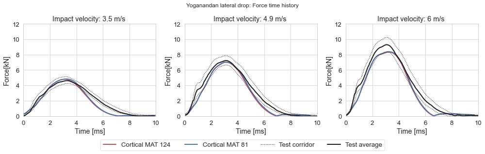
All specimens were tested for 3.5 m/s, 4.9 m/s and 6 m/s.
Force time history curves along with the corridors provided in the litrature
velocity [m/s] |
Specimens |
Average Head mass [kg] |
|---|---|---|
3.5 |
1,2,3,4,5,7,8,9 |
3.52 |
4.9 |
1,2,3,5,6,7,8,9,10 |
3.71 |
6 |
1,2,3,5,6,7,8,9,10 |
3.71 |
biomechanical data of the peak force, deflection, and energy for the highest impact velocity test for each specimen is also given,
ID |
Velocity [m/s] |
Force [N] |
Displacement [mm] |
|---|---|---|---|
1 |
5.99 |
9374.9 |
13.6 |
2 |
6.92 |
9917.6 |
16.2 |
3 |
6.92 |
8836.2 |
16.1 |
4 |
4.89 |
5556.4 |
10.4 |
5 |
5.99 |
6929.3 |
14.0 |
6 |
6.92 |
7678.3 |
16.1 |
7 |
7.74 |
7448.7 |
19.1 |
8 |
6.92 |
9128.1 |
15.0 |
9 |
6.47 |
9608.8 |
15.6 |
10 |
5.99 |
9261.6 |
14.3 |
Reconstruction#
VIVA+ head repositioned using global transforms positioned for lateral drop.
The skull was dropped into 40 durometer padding resting on a rigid load cell.
40 durometer padding mdelled using
MAT63_CRUSHABLE_FOAMwith mass density \(4230 kg/m^3\), Youngs modulus: \(9 Mpa\) and Poissons ratio \(0.43\) [3].Stress-strain curve for tested IMPAXX \(^{TM}\) foam [4] is incoperated in the material model in LS-DYNA.
*CONTACT_AUTOMATIC_SURFACETO_SURFACE is defined between the skull and the pad with a static friction coefficient 0.7.
Responses recorded#
TIme history of the reaction force at the rigid boundary surface is measured.
The reference values from the paper were digitalised and are incuded in the notebook. The data corresponds to the unnormalised corridors.
modelling references#
Slik G, Vogel G, Chawda V, Automotive D. Material model validation of a high efficient energy absorbing foam. In Proceedings of the 5th LS-DYNA Forum 2006 Oct 12. Materials Engineering Centre. Article
Other Notes for simulation#
The mass of the model was matched to the tests using
*ELEMENT_MASS_NODEcard to add masses.
Material cards used in skull bone#
Trabecular bone modelled with MAT124 MAT_PLASTICITY_COMPRESSION_TENSION based on compression and tension stress-strain curves from tests done by Boruah (2013)
Cortical bone available with two types material cards based tests done by Wood (1971)
MAT124 MAT_PLASTICITY_COMPRESSION_TENSION
MAT81 MAT_PLASTICITY_WITH_DAMAGE
Yoganandan (2003)#
Show code cell source
fig_fd, axs = plt.subplots(nrows=1, ncols=3,figsize=(14, 4))
fig_fd.suptitle('Yoganandan lateral drop: Force time history')
Tests=["drop_3.5","drop_4.9","drop_6"]
for i in range(3):
    axs[i].set_ylabel('Force[kN]');
    axs[i].set_xlabel('Time [ms]');
    axs[i].set_xlim(0,10)
    axs[i].set_ylim(0,12)

axs[0].set_title('Impact velocity: 3.5 m/s ')
axs[1].set_title('Impact velocity: 4.9 m/s ')
axs[2].set_title('Impact velocity: 6 m/s ')

axs[0].plot(pd.DataFrame(sim_results[version[0],Tests[0]]).SETUP.Force.time-1.0,pd.DataFrame(sim_results[version[0],Tests[0]]).SETUP.Force.force, linewidth=2,color='r',label='Cortical MAT 124 ')
axs[0].plot(pd.DataFrame(sim_results[version[1],Tests[0]]).SETUP.Force.time-1.0,pd.DataFrame(sim_results[version[1],Tests[0]]).SETUP.Force.force, linewidth=2,color='b',label='Cortical MAT 81')
axs[0].plot(exp_test1_cor.u_time*1000,exp_test1_cor.u_force/1000,':k',label='Test corridor')
axs[0].plot(exp_test1_cor.l_time*1000,exp_test1_cor.l_force/1000,':k')
axs[0].plot(exp_test1[0]*1000,exp_test1[1]/1000,'k', linewidth=2,label='Test average')


axs[1].plot(pd.DataFrame(sim_results[version[0],Tests[1]]).SETUP.Force.time-1.5,pd.DataFrame(sim_results[version[0],Tests[1]]).SETUP.Force.force, linewidth=2,color='r')
axs[1].plot(pd.DataFrame(sim_results[version[1],Tests[1]]).SETUP.Force.time-1.5,pd.DataFrame(sim_results[version[1],Tests[1]]).SETUP.Force.force, linewidth=2,color='b')
axs[1].plot(exp_test2_cor.u_time*1000,exp_test2_cor.u_force/1000,':k')
axs[1].plot(exp_test2_cor.l_time*1000,exp_test2_cor.l_force/1000,':k')
axs[1].plot(exp_test2[0]*1000,exp_test2[1]/1000,'k', linewidth=2)

axs[2].plot(pd.DataFrame(sim_results[version[0],Tests[2]]).SETUP.Force.time-1.3,pd.DataFrame(sim_results[version[0],Tests[2]]).SETUP.Force.force, linewidth=2,color='r')
axs[2].plot(pd.DataFrame(sim_results[version[1],Tests[2]]).SETUP.Force.time-1.3,pd.DataFrame(sim_results[version[1],Tests[2]]).SETUP.Force.force, linewidth=2,color='b')
axs[2].plot(exp_test3_cor.u_time*1000,exp_test3_cor.u_force/1000,':k')
axs[2].plot(exp_test3_cor.l_time*1000,exp_test3_cor.l_force/1000,':k')
axs[2].plot(exp_test3[0]*1000,exp_test3[1]/1000,'k', linewidth=2)

fig_fd.legend(loc="lower center", bbox_to_anchor=(0.5,- 0.1), ncol=4);
fig_fd.tight_layout()
fig_fd.savefig(os.path.join(figures_dir, 'Force_time_corridor.jpg'), transparent=False, dpi=600, bbox_inches="tight")
Yoganandan (2004): IRCOBI#
Show code cell source
fig_irb, axs = plt.subplots(nrows=2, ncols=5, figsize=(20, 6))
fig_irb.suptitle('Force time history',fontsize=18)
Tests=["test_1","test_2","test_3","test_4","test_5","test_6","test_7","test_8","test_9","test_10"]
names=["44y | 5.99 m/s | 4.37kg","56y | 6.92 m/s | 4.26kg","71y | 6.92 m/s | 3.72kg","68y | 4.89 m/s | 2.67kg *","77y | 5.99 m/s | 3.54kg","65y | 6.92 m/s | 3.58kg"
            ,"87y | 7.74 m/s | 2.35kg *","30y | 6.92 m/s | 3.35kg","70y | 6.47 m/s | 3.87kg","59y | 5.99 m/s | 4.43kg"]
# experiment data
exp_loads=[9.3749,	9.9176	,8.8362,	5.5564,	6.9293,	7.6783	,7.4487,	9.1281,	9.6088,	9.2616]
i=0
for x in range(2):
    for y in range(5):
        axs[x,y].plot(pd.DataFrame(sim_results[version[0],Tests[i]]).SETUP.Force.time,pd.DataFrame(sim_results[version[0],Tests[i]]).SETUP.Force.force,'r', linewidth=2,label='MAT 124 ')
        axs[x,y].plot(pd.DataFrame(sim_results[version[1],Tests[i]]).SETUP.Force.time,pd.DataFrame(sim_results[version[1],Tests[i]]).SETUP.Force.force, linewidth=2,color='b',label='MAT 81')
        axs[x,y].axhline(y=exp_loads[i], linestyle='--',color='k',linewidth=2)
        axs[x,y].set_title('{}'.format(names[i]))
        axs[x,y].set_xlim([0,10])
        axs[x,y].set_ylim([0,12])
        i=i+1
fig_irb.legend(["Cortical: MAT 124","Cortical: MAT 81","Test **"], bbox_to_anchor=(0.65,0), ncol=4);
fig_irb.text(0, 0.45,'Force[kN]', ha='center', rotation='vertical',fontsize=16);
fig_irb.text(0.5, 0,'Time [ms]', ha='center',fontsize=16);
plt.figtext(0.85,-0.015, "* simulation mass ~ 3.14kg",fontsize=14, style='italic',color='grey')
plt.figtext(0.84,-0.055, "** Peak loads reported in the test",fontsize=14, style='italic',color='grey')
fig_irb.tight_layout()
#save figure
fig_irb.savefig(os.path.join(figures_dir, 'Force_time_IRCOBI.jpg'), transparent=False, dpi=600, bbox_inches="tight")
