Proximal femur (Ariza 2015)

Validation model information

• Performed by: Alexander Schubert / Nico Erlinger

• Reviewed by: Corina Klug

• Current Responsible:

Added to VIVA+ Validation Catalog on: 2022-10-21

Last modified: 2023-03-13

Model version (this notebook run for): 0.3.2

© 2019-2023, OpenVT Organization (OVTO)

Available openly under under Creative Commons Attribution 4.0 International License

Reference

A. Schubert, N. Erlinger, C. Leo, J. Iraeus, J. John, C. Klug (2021): “Development of a 50th Percentile Female Femur Model”, IRCOBI conference proceedings, http://www.ircobi.org/wordpress/downloads/irc21/pdf-files/2138.pdf

Experiments by Ariza (2014) and Ariza et al. (2015)

Ariza, O.; Gilchrist, S.; Widmer, R. P.; Guy, P.; Ferguson, S. J.; Cripton, P. A.; Helgason, B., Comparison of explicit finite element and mechanical simulation of the proximal femur during dynamic drop-tower testing, Journal of biomechanics, Vol. 48, 2015.

Ariza, O. A novel approach to finite element analysis of hip fractures due to sideways falls Master Thesis University of Britisch Columbia (Vancouver), 2014.

Summary

14 dynamic drop tower tests on the proximal femur were replicated by prescribing the vertical motion of the upper potting.

Information on the subjects/specimens

Specimen	Bone density	Donor age
H1167L	normal	50
H1365R	osteoporotic	71
H1366R	normal	73
H1368R	osteoporotic	70
H1369L	osteoporotic	69
H1372R	normal	79
H1373R	osteoporotic	76
H1374R	osteoporotic	78
H1375L	normal	83
H1376L	normal	79
H1377R	osteoporotic	80
H1380R	normal	71
H1381R	osteoporotic	92
H1382L	osteoporotic	96

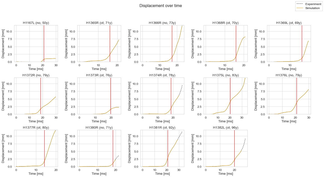
Loading and Boundary Conditions

The displacement-time histories from the diagrams published by Ariza (2014) were digitised with WebPlotDigitizer v4.4 (https://automeris.io/WebPlotDigitizer).

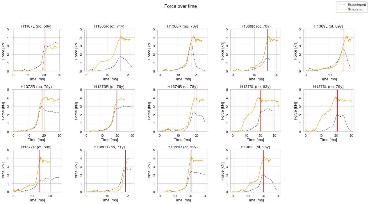
Experimental responses

The force-time histories, published by Ariza (2014) were digitised with WebPlotDigitizer v4.4.

Other notes for simulation

Notes on implementation and iterations during the implementation of validation simulations.

Show code cell content Hide code cell content

simulation_list = ["H1167L", "H1365R", "H1366R", "H1368R", "H1369L", "H1372R", "H1373R", 
                   "H1374R", "H1375L", "H1376L", "H1377R", "H1380R", "H1381R", "H1382L"]


name ='Name_of_person'
date = datetime.date.today().strftime('%Y-%m-%d')
dynasaur_output_file_name = 'Dynasaur_output.csv'

Plots

Show code cell source Hide code cell source

simulation_list = ["H1167L", "H1365R", "H1366R", "H1368R", "H1369L", "H1372R", "H1373R", 
                   "H1374R", "H1375L", "H1376L", "H1377R", "H1380R", "H1381R", "H1382L"]

simulation_titles = ['H1167L (no, 50y)', 
                     'H1365R (ot, 71y)',
                     'H1366R (no, 73y)',
                     'H1368R (ot, 70y)',
                     'H1369L (ot, 69y)',
                     'H1372R (no, 79y)',
                     'H1373R (ot, 76y)',
                     'H1374R (ot, 78y)',
                     'H1375L (no, 83y)',
                     'H1376L (no, 79y)',
                     'H1377R (ot, 80y)',
                     'H1380R (no, 71y)',
                     'H1381R (ot, 92y)',
                     'H1382L (ot, 96y)']

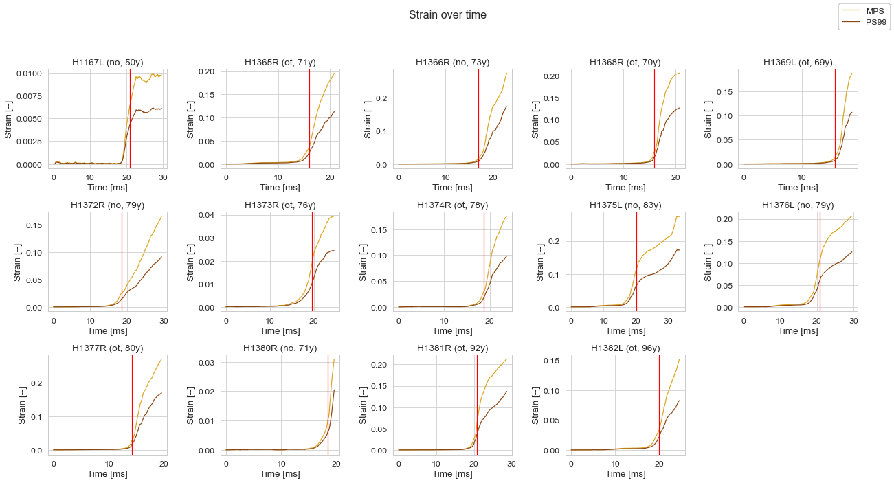
time_for_strain_eval = [21.0, 16.0, 17.0, 15.9, 15.7, 18.5, 19.6, 18.6, 20.2, 20.8, 14.2, 18.4, 20.8, 20.0]

experiment_data_dir = 'data/experiment/'
#processed_data_dir = f'data/processed/{date}_{name}'
processed_data_dir = f'data/processed/2022-10-19_Name_of_person'

def create_subplots(experiment_file, figure_title, sim_x_data, sim_y_data, sim_x_data2, sim_y_data2, 
                    sim_name1_legend, sim_name2_legend, x_label, y_label, x_lim, y_lim, sign_swap_exp_data, 
                    sign_swap_sim_data, filename_save):
    figure, ((ax1, ax2, ax3, ax4, ax5), (ax6, ax7, ax8, ax9, ax10), (ax11, ax12, ax13, ax14, ax15)) = plt.subplots(
        3,5, figsize=(18,10))
    axs = [ax1, ax2, ax3, ax4, ax5, ax6, ax7, ax8, ax9, ax10, ax11, ax12, ax13, ax14, ax15]
    figure.suptitle(figure_title)
    figure.delaxes(axs[14])
    figure.tight_layout(pad=3)
    
    if experiment_file is not None:
        experimental_data = pd.read_csv(experiment_data_dir + experiment_file, delimiter=';', header=[0], decimal='.')   
    
    plot_style_experimental = {"linestyle" :'--', "color" : 'black',  "alpha" : 0.7}
    plot_style_simulation = {"linestyle" :'-', "color" : 'goldenrod'}
    plot_style_simulation2 = {"linestyle" :'-', "color" : 'saddlebrown'}
    
    counter = 0
    
    for i in simulation_list:
        if experiment_file is not None:
            x_data = experimental_data['Time'].values
            y_data = experimental_data[i].values * sign_swap_exp_data
            y_data = experimental_data[i].values
            axs[counter].plot(x_data, y_data, **plot_style_experimental)
            figure.legend(('Experiment', 'Simulation'), loc='upper right')
        
        processed_data_path = os.path.join(processed_data_dir, i).replace('\\', '/')
        simData = pd.read_csv(os.path.join(processed_data_path, dynasaur_output_file_name), 
                                    delimiter=';', na_values='-', header = [0,1,2,3])
        x_data = simData[sim_x_data]
        y_data = simData[sim_y_data]
        y_data = y_data * sign_swap_sim_data
        axs[counter].plot(x_data, y_data, **plot_style_simulation)
        
        if sim_x_data2 and sim_x_data2 is not None:         
            x_data = simData[sim_x_data2]
            y_data = simData[sim_y_data2]
            y_data = y_data * sign_swap_sim_data
            axs[counter].plot(x_data, y_data, **plot_style_simulation2)
            figure.legend((sim_name1_legend, sim_name2_legend), loc='upper right')
        
        axs[counter].set(xlabel=x_label)
        axs[counter].set_ylabel(y_label)       
        axs[counter].set_ylim(y_lim)    
        axs[counter].title.set_text(simulation_titles[counter])
        axs[counter].axvline(x=time_for_strain_eval[counter], color='red')
                      
        counter += 1

    figure.savefig(filename_save, format='svg', bbox_inches='tight')

    
figure_title = 'Force over time'    
experiment_file = 'ariza_et_al_2015_force_time.csv'
sim_x_data = 'FEMUR', 'Impactor_rcforc_z', 'time'
sim_y_data = 'FEMUR', 'Impactor_rcforc_z', 'force'
sim_x_data2 = None
sim_y_data2 = None
sim_name1_legend = None
sim_name2_legend = None
x_label = 'Time [ms]'
y_label = 'Force [kN]'
x_lim = [0, 30]
y_lim = [0, 5]
sign_swap_exp_data = 1
sign_swap_sim_data = 1
filename_save = 'results/figures/Ariza_force_time.svg'    
create_subplots(experiment_file, figure_title, sim_x_data, sim_y_data, sim_x_data2, sim_y_data2, sim_name1_legend, 
                sim_name2_legend, x_label, y_label, x_lim, y_lim, sign_swap_exp_data, sign_swap_sim_data, filename_save)


figure_title = 'Displacement over time'
experiment_file = 'ariza_et_al_2015_impactor_displacement.csv'
sim_x_data = 'FEMUR', 'Impactor_nodout_z', 'time'
sim_y_data = 'FEMUR', 'Impactor_nodout_z', 'displacement'
sim_x_data2 = None
sim_y_data2 = None
sim_name1_legend = None
sim_name2_legend = None
x_label = 'Time [ms]'
y_label = 'Displacement [mm]'
x_lim = [0, 30]
y_lim = [0, 12]
sign_swap_exp_data = 1
sign_swap_sim_data = -1
filename_save = 'results/figures/Ariza_displacement_time.svg'    
create_subplots(experiment_file, figure_title, sim_x_data, sim_y_data, sim_x_data2, sim_y_data2, sim_name1_legend, 
                sim_name2_legend, x_label, y_label, x_lim, y_lim, sign_swap_exp_data, sign_swap_sim_data, filename_save)


figure_title = 'Strain over time'
experiment_file = None
sim_x_data = 'BONES', 'Femur_Cortical_L_MPS_history', 'time'
sim_y_data = 'BONES', 'Femur_Cortical_L_MPS_history', 'strain'
sim_x_data2 = 'BONES', 'Femur_Cortical_L_PS99_history', 'time'
sim_y_data2 = 'BONES', 'Femur_Cortical_L_PS99_history', 'strain'
sim_name1_legend = 'MPS'
sim_name2_legend = 'PS99'
x_label = 'Time [ms]'
y_label = 'Strain [--]'
x_lim = [0, 30]
y_lim = None
sign_swap_exp_data = 1
sign_swap_sim_data = 1
filename_save = 'results/figures/Ariza_strain_time.svg'    
create_subplots(experiment_file, figure_title, sim_x_data, sim_y_data, sim_x_data2, sim_y_data2, sim_name1_legend, 
                sim_name2_legend, x_label, y_label, x_lim, y_lim, sign_swap_exp_data, sign_swap_sim_data, filename_save)


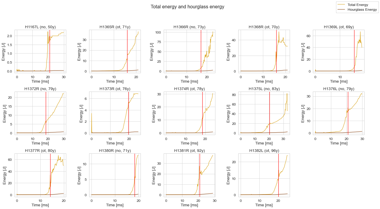
figure_title = 'Total energy and hourglass energy'
experiment_file = None
sim_x_data = 'MODEL', 'Total_Energy', 'time'
sim_y_data = 'MODEL', 'Total_Energy', 'energy'
sim_x_data2 = 'MODEL', 'Hourglass_Energy', 'time'
sim_y_data2 = 'MODEL', 'Hourglass_Energy', 'energy'
sim_name1_legend = 'Total Energy'
sim_name2_legend = 'Hourglass Energy'
x_label = 'Time [ms]'
y_label = 'Energy [J]'
x_lim = [0, 30]
y_lim = None
sign_swap_exp_data = 1
sign_swap_sim_data = 1
filename_save = 'results/figures/Ariza__total_energy__hourglass_energy__time.svg'    
create_subplots(experiment_file, figure_title, sim_x_data, sim_y_data, sim_x_data2, sim_y_data2, sim_name1_legend, 
                sim_name2_legend, x_label, y_label, x_lim, y_lim, sign_swap_exp_data, sign_swap_sim_data, filename_save)


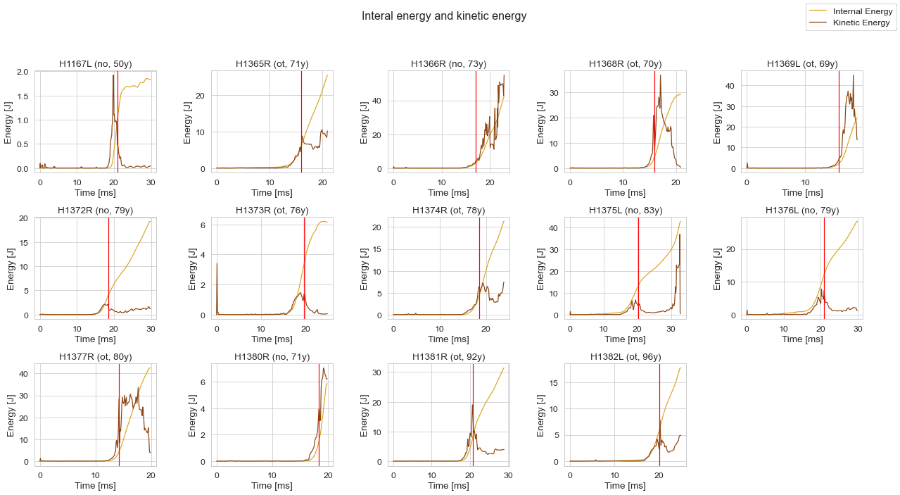
figure_title = 'Interal energy and kinetic energy'
experiment_file = None
sim_x_data = 'MODEL', 'Internal_Energy', 'time'
sim_y_data = 'MODEL', 'Internal_Energy', 'energy'
sim_x_data2 = 'MODEL', 'Kinetic_Energy', 'time'
sim_y_data2 = 'MODEL', 'Kinetic_Energy', 'energy'
sim_name1_legend = 'Internal Energy'
sim_name2_legend = 'Kinetic Energy'
x_label = 'Time [ms]'
y_label = 'Energy [J]'
x_lim = [0, 30]
y_lim = None
sign_swap_exp_data = 1
sign_swap_sim_data = 1
filename_save = 'results/figures/Ariza__interal_energy__kinetic_energy__time.svg'    
create_subplots(experiment_file, figure_title, sim_x_data, sim_y_data, sim_x_data2, sim_y_data2, sim_name1_legend, 
                sim_name2_legend, x_label, y_label, x_lim, y_lim, sign_swap_exp_data, sign_swap_sim_data, filename_save)

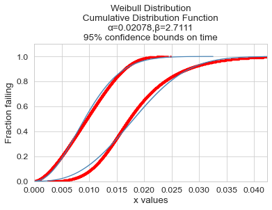
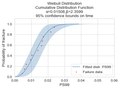
Injury Risk Curves

Show code cell source Hide code cell source

import os
import scipy
import numpy as np
import pandas as pd
import matplotlib.pyplot as plt
import scipy.stats as stats
from autograd import jacobian as jac
import autograd.numpy as anp
from reliability.Distributions import Weibull_Distribution
from reliability.Fitters import Fit_Weibull_2P, Fit_Weibull_3P
from reliability.Probability_plotting import plot_points
import matplotlib.pyplot as plt


df_strains = pd.read_csv('data/processed/strain_sheet_for_IRC.csv', sep = ";")


def confidence_interval_weibul_time(CI, alpha, beta, Cov_alpha_beta, alpha_SE, beta_SE):
    Y= np.arange(0.0001,0.9999,0.0001)
    Z = -stats.norm.ppf((1 - CI) / 2)  # converts CI to Z
    v_lower = v(Y, alpha, beta) - Z * (var_v(Y, alpha, beta, Cov_alpha_beta, alpha_SE, beta_SE) ** 0.5)
    v_upper = v(Y, alpha, beta) + Z * (var_v(Y, alpha, beta, Cov_alpha_beta, alpha_SE, beta_SE) ** 0.5)
    t_lower = np.exp(v_lower)  # transform back from ln(t)
    t_upper = np.exp(v_upper) 
    yy = 1 - Y
    df = pd.DataFrame(columns=('yy', 't_lower', 't_upper'))
    df.yy = yy
    df.t_lower = t_lower
    df.t_upper = t_upper
    #print(df)
    print('------Lower----------')
    weibull_fit_lower = Fit_Weibull_2P(failures=list(df.t_lower), show_probability_plot=False, print_results=True, 
                                       CI=0.95, CI_type="time")
    print('------Upper----------')
    weibull_fit_upper = Fit_Weibull_2P(failures=list(df.t_upper), show_probability_plot=False, print_results=True, 
                                       CI=0.95, CI_type="time")
    weibull_fit_lower.distribution.CDF(label='Fitted distribution', color='steelblue')
    plot_points(failures=list(df.t_lower),func='CDF',label='Failure data', color='red', alpha=0.7)
    weibull_fit_upper.distribution.CDF(label='Fitted distribution', color='steelblue')
    plot_points(failures=list(df.t_upper),func='CDF',label='Failure data', color='red', alpha=0.7)
    plt.show()

def u(t, alpha, beta):  # u = ln(-ln(R))
    return beta * (anp.log(t) - anp.log(alpha))  # weibull SF linearized

def v(R, alpha, beta):  # v = ln(t)
    return (1 / beta) * anp.log(-anp.log(R)) + anp.log(
        alpha
    )  # weibull SF rearranged for t
            
def var_u(v, alpha, beta, Cov_alpha_beta, alpha_SE, beta_SE):  # v is time
    du_da = jac(u, 1)  # derivative wrt alpha (bounds on reliability)
    du_db = jac(u, 2)  # derivative wrt beta (bounds on reliability)
    return (
        du_da(v, alpha, beta) ** 2 * alpha_SE ** 2
        + du_db(v, alpha, beta) ** 2 * beta_SE ** 2
        + 2
        * du_da(v, alpha, beta)
        * du_db(v, alpha, beta)
        * Cov_alpha_beta
    )

def var_v(u, alpha, beta, Cov_alpha_beta, alpha_SE, beta_SE):  # u is reliability
    dv_da = jac(v, 1)  # derivative wrt alpha (bounds on time)
    dv_db = jac(v, 2)  # derivative wrt beta (bounds on time)
    return (
        dv_da(u, alpha, beta) ** 2 * alpha_SE ** 2
        + dv_db(u, alpha, beta) ** 2 * beta_SE ** 2
        + 2
        * dv_da(u, alpha, beta)
        * dv_db(u, alpha, beta)
        * Cov_alpha_beta
      )

strains = ['MPS', 'PS99']
for i in range(len(strains)):
    print('--------------------------------------------------------------------------------------')
    print (strains[i])
    strain_list = list(df_strains[strains[i]])    
    print('--------------------------------------------------------------------------------------')
    weibull_fit = Fit_Weibull_2P(failures=strain_list, show_probability_plot=False, print_results=True, 
                                 CI=0.95, CI_type="time")
    label = 'Fitted distr. ' + strains[i]
    weibull_fit.distribution.CDF(label=label, color='steelblue')
    plot_points(failures=strain_list, func='CDF', label='Failure data', color='red',alpha=0.7)
    plt.legend()
    plt.xlabel(strains[i])
    plt.xlim([0, 0.06])
    plt.ylabel('Probability of fracture')
    filepath = 'results/figures/weibull_{}_fit.svg'.format(strains[i])
    plt.savefig(filepath, format='svg', bbox_inches='tight')
    plt.show()
    confidence_interval_weibul_time(0.95, weibull_fit.alpha, weibull_fit.beta, weibull_fit.Cov_alpha_beta, 
                                    weibull_fit.alpha_SE, weibull_fit.beta_SE)

--------------------------------------------------------------------------------------
MPS
--------------------------------------------------------------------------------------
Results from Fit_Weibull_2P (95% CI):
Analysis method: Maximum Likelihood Estimation (MLE)
Optimizer: TNC
Failures / Right censored: 11/0 (0% right censored) 

Parameter  Point Estimate  Standard Error  Lower CI  Upper CI
    Alpha       0.0251501      0.00303181 0.0198577 0.0318531
     Beta         2.62164        0.664574   1.59514   4.30873 

Goodness of fit    Value
 Log-likelihood  35.8516
           AICc -66.2032
            BIC -66.9074
             AD  1.42996 

------Lower----------
Results from Fit_Weibull_2P (95% CI):
Analysis method: Maximum Likelihood Estimation (MLE)
Optimizer: TNC
Failures / Right censored: 9998/0 (0% right censored) 

Parameter  Point Estimate  Standard Error  Lower CI  Upper CI
    Alpha       0.0188615     8.70578e-05 0.0186917 0.0190329
     Beta          2.2698       0.0185938   2.23365   2.30654 

Goodness of fit    Value
 Log-likelihood  34433.1
           AICc -68862.2
            BIC -68847.8
             AD  45.4323 

------Upper----------
Results from Fit_Weibull_2P (95% CI):
Analysis method: Maximum Likelihood Estimation (MLE)
Optimizer: TNC
Failures / Right censored: 9998/0 (0% right censored) 

Parameter  Point Estimate  Standard Error  Lower CI  Upper CI
    Alpha        0.033667      0.00011894 0.0334347 0.0339009
     Beta         3.00049       0.0215959   2.95846   3.04312 

Goodness of fit    Value
 Log-likelihood  31481.4
           AICc -62958.7
            BIC -62944.3
             AD  101.785 

--------------------------------------------------------------------------------------
PS99
--------------------------------------------------------------------------------------
Results from Fit_Weibull_2P (95% CI):
Analysis method: Maximum Likelihood Estimation (MLE)
Optimizer: TNC
Failures / Right censored: 11/0 (0% right censored) 

Parameter  Point Estimate  Standard Error  Lower CI  Upper CI
    Alpha        0.015083      0.00203068 0.0115848 0.0196376
     Beta         2.35987        0.575181    1.4636   3.80501 

Goodness of fit    Value
 Log-likelihood  40.8492
           AICc -76.1984
            BIC -76.9026
             AD  1.33966 

------Lower----------
Results from Fit_Weibull_2P (95% CI):
Analysis method: Maximum Likelihood Estimation (MLE)
Optimizer: TNC
Failures / Right censored: 9998/0 (0% right censored) 

Parameter  Point Estimate  Standard Error  Lower CI  Upper CI
    Alpha       0.0109873     5.63325e-05 0.0108774 0.0110983
     Beta         2.04409       0.0166948   2.01163   2.07708 

Goodness of fit    Value
 Log-likelihood  39103.2
           AICc -78202.5
            BIC -78188.1
             AD  39.3013 

------Upper----------
Results from Fit_Weibull_2P (95% CI):
Analysis method: Maximum Likelihood Estimation (MLE)
Optimizer: TNC
Failures / Right censored: 9998/0 (0% right censored) 

Parameter  Point Estimate  Standard Error  Lower CI  Upper CI
    Alpha       0.0207839     8.12327e-05 0.0206253 0.0209437
     Beta         2.71109       0.0196152   2.67292   2.74981 

Goodness of fit    Value
 Log-likelihood  35444.9
           AICc -70885.8
            BIC -70871.4
             AD  87.3722