Pedestrian (Paas 2015)#
Postprocessing of femur shaft validations based on Paas et al. 2015
Performed by: Nico Erlinger
Reviewed by: Corina Klug
Added to VIVA+ Validation Catalog on: 2022-10-21
Version |
Date |
Performed by |
LS-Dyna |
|---|---|---|---|
0.3.2 |
2022-10-19 |
Nico Erlinger |
9.3.1 |
1.1.0 |
2024-06-04 |
Corina Klug |
12.0.0. |
© 2019-2024, OpenVT Organization (OVTO)
Available openly under under Creative Commons Attribution 4.0 International License 
References#
Experimental data#
Paas, R., Masson, C., and Davidsson, J. (2015). Head boundary conditions in pedestrian crashes with passenger cars: Six-degrees-of-freedom post-mortem human subject responses. International Journal of Crashworthiness 20, 547–559. doi: 10.1080/13588265.2015.1060731
Paas, R., Östh, J., and Davidsson, J. (2015). “Which Pragmatic Finite Element Human Body Model Scaling Technique Can Most Accurately Predict Head Impact Conditions in Pedestrian-Car Crashes?” in 2015 IRCOBI Conference Proceedings, ed. International Research Council on the Biomechanics of Injury (IRCOBI), 546–576. http://www.ircobi.org/wordpress/downloads/irc15/pdf_files/64.pdf
VIVA+ validation#
Manuscript currently under preparation
Information on the subjects/specimens#
PMHS |
Sex |
Height [cm] |
Weight [kg] |
Age [yr] |
Scale factor z (height) |
Scale factor xand y (weight) |
|---|---|---|---|---|---|---|
PM01 |
m |
172 |
69 |
72 |
0.98 |
0.96 |
PF02 |
f |
154 |
47 |
85 |
0.95 |
0.88 |
PM03 |
m |
175 |
88 |
61 |
1.00 |
1.08 |
PM04 |
m |
179 |
81 |
83 |
1.02 |
1.02 |
PM05 |
m |
174 |
68 |
89 |
0.99 |
0.94 |
Postures
PM01 |
PF02 |
PM03 |
PM04 |
PM05 |
|||||||
|---|---|---|---|---|---|---|---|---|---|---|---|
Experiment [°] |
pos. VIVA+ [°] |
Experiment [°] |
pos. VIVA+ [°] |
Experiment [°] |
pos. VIVA+ [°] |
Experiment [°] |
pos. VIVA+ [°] |
Experiment [°] |
pos. VIVA+ [°] |
||
side view |
Right lower leg |
-10 |
-5 |
-1 |
-2 |
-12 |
-11 |
-8 |
-6 |
-3 |
0 |
Right upper leg |
6 |
2 |
7 |
6 |
1 |
2 |
12 |
9 |
13 |
8 |
|
Left lower leg |
-15 |
-15 |
-12 |
-11 |
-15 |
-16 |
-37 |
-33 |
-29 |
-29 |
|
Left upper leg |
6 |
1 |
11 |
7 |
1 |
1 |
2 |
4 |
10 |
5 |
|
Right lower arm |
4 |
8 |
10 |
7 |
9 |
11 |
14 |
12 |
12 |
18 |
|
Right upper arm |
-8 |
-6 |
-2 |
-3 |
-1 |
-6 |
-5 |
-6 |
-1 |
-6 |
|
Left lower arm |
44 |
40 |
17 |
17 |
22 |
23 |
32 |
30 |
11 |
13 |
|
Left upper arm |
-1 |
-1 |
3 |
3 |
8 |
6 |
1 |
6 |
4 |
6 |
|
front view |
Right lower leg |
1 |
2 |
1 |
6 |
10 |
15 |
-6 |
-9 |
2 |
3 |
Right upper leg |
-9 |
-7 |
0 |
2 |
8 |
7 |
1 |
4 |
4 |
3 |
|
Left lower leg |
-8 |
-11 |
12 |
13 |
6 |
6 |
10 |
10 |
2 |
3 |
|
Left upper leg |
-7 |
-9 |
-2 |
-6 |
4 |
9 |
1 |
6 |
-4 |
-5 |
|
Right lower arm |
-7 |
-9 |
2 |
2 |
-10 |
-7 |
7 |
4 |
-10 |
-8 |
|
Right upper arm |
9 |
9 |
8 |
7 |
7 |
8 |
5 |
8 |
15 |
12 |
|
Left lower arm |
22 |
25 |
-3 |
1 |
12 |
11 |
13 |
17 |
8 |
7 |
|
Left upper arm |
-25 |
-23 |
-8 |
-6 |
-4 |
-8 |
-5 |
-8 |
16 |
15 |
|
Pelvis |
89 |
90 |
91 |
90 |
89 |
89 |
91 |
90 |
89 |
89 |
|
Upper body centreline |
-1 |
0 |
1 |
0 |
1 |
0 |
0 |
0 |
0 |
0 |
|
Shoulder |
90 |
89 |
93 |
90 |
91 |
90 |
91 |
90 |
95 |
90 |
Loading and Boundary Conditions#
The displacement-time histories from the diagrams published by Paas et al. (2015) were digitised with WebPlotDigitizer v4.4 (https://automeris.io/WebPlotDigitizer).
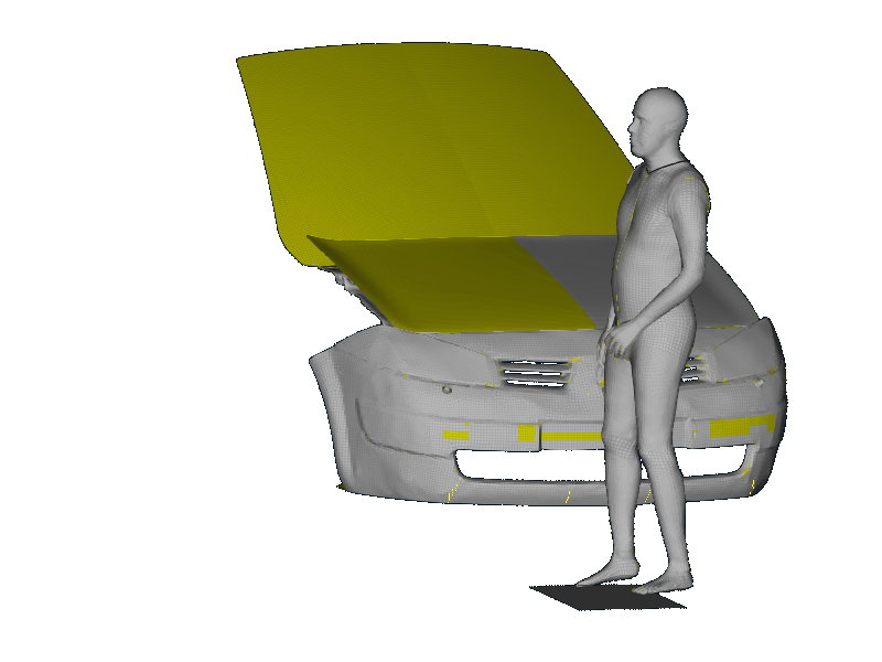
The setup of PM01 is shown exemplary below.
Experimental responses#
Currently only trajectories are compared
Simulation metadata#
Function for plotting#
Results#
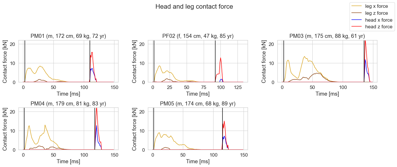
Head impact times#
Show code cell source
hit_array=calculate_head_impact_time(
sim_x_data_leg = ('HBM', 'HBM_Leg_Vehicle_Contact_Transducer_x_force', 'time'),
sim_y_data_leg = ('HBM', 'HBM_Leg_Vehicle_Contact_Transducer_x_force', 'force'),
sim_x_data_head = ('HBM', 'HBM_Head_Vehicle_Contact_Transducer_z_force', 'time'),
sim_y_data_head = ('HBM', 'HBM_Head_Vehicle_Contact_Transducer_z_force', 'force')
)

head_time_exp = [120, 102, 162, 120, 111]
hit_df = pd.DataFrame(hit_array, columns=['Simulation', 'First leg contact [ms]', 'First head contact [ms]', 'Simulation HIT [ms]'])
hit_df['Experimental HIT [ms]'] = np.array(head_time_exp)
hit_df.interpolate()
display(hit_df)

create_subplots(
figure_title = 'Head and leg contact force',
sim_x_data = ('HBM', 'HBM_Leg_Vehicle_Contact_Transducer_x_force', 'time'),
sim_y_data = ('HBM', 'HBM_Leg_Vehicle_Contact_Transducer_x_force', 'force'),
sim_x_data2 = ('HBM', 'HBM_Leg_Vehicle_Contact_Transducer_z_force', 'time'),
sim_y_data2 = ('HBM', 'HBM_Leg_Vehicle_Contact_Transducer_z_force', 'force'),
sim_x_data3 = ('HBM', 'HBM_Head_Vehicle_Contact_Transducer_x_force', 'time'),
sim_y_data3 = ('HBM', 'HBM_Head_Vehicle_Contact_Transducer_x_force', 'force'),
sim_x_data4 = ('HBM', 'HBM_Head_Vehicle_Contact_Transducer_z_force', 'time'),
sim_y_data4 = ('HBM', 'HBM_Head_Vehicle_Contact_Transducer_z_force', 'force'),
sim_name1_legend = 'leg x force',
sim_name2_legend = 'leg z force',
sim_name3_legend = 'head x force',
sim_name4_legend = 'head z force',
x_label = 'Time [ms]',
y_label = 'Contact force [kN]',
vertical_line1 = list(map(float, (hit_df['First leg contact [ms]'].tolist()))),
vertical_line2 = list(map(float, (hit_df['First head contact [ms]'].tolist()))),
x_lim = [0, 150],
y_lim = [0, 22],
)
| Simulation | First leg contact [ms] | First head contact [ms] | Simulation HIT [ms] | Experimental HIT [ms] | |
|---|---|---|---|---|---|
| 0 | PM01 | 3.0 | 110.0 | 107 | 120 |
| 1 | PF02 | 2.0 | 92.0 | 90 | 102 |
| 2 | PM03 | 3.0 | 135.0 | 132 | 162 |
| 3 | PM04 | 2.0 | 118.0 | 116 | 120 |
| 4 | PM05 | 2.0 | 115.0 | 113 | 111 |
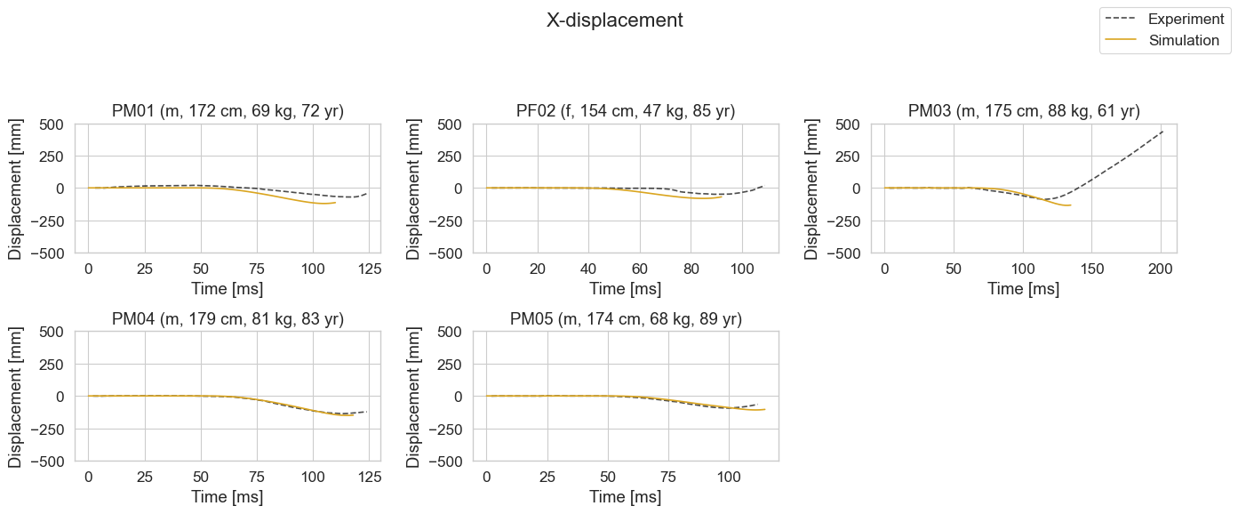
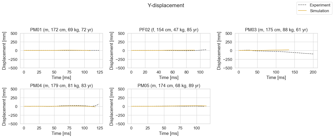
Head COG displacements#
Show code cell source
create_subplots(
figure_title = 'X-displacement',
offset_exp_data_x = list(map(float, (hit_df['First leg contact [ms]'].tolist()))),
cut_sim_data = list(map(float, (hit_df['First head contact [ms]'].tolist()))),
sim_x_data = ('HEAD', 'x-displacement', 'time'),
sim_y_data = ('HEAD', 'x-displacement', 'displacement'),
exp_x_data = ('Head', 'time'),
exp_y_data = ('Head', 'x-displacement'),
sim_name1_legend = 'Simulation',
exp_name1_legend = 'Experiment',
x_label = 'Time [ms]',
y_label = 'Displacement [mm]',
x_lim = [0, 200],
y_lim = [-500, 500],
filename_save = 'results/figures/VIVA+_Paas_et_al_2015_x-displacement_time.svg'
)
create_subplots(
figure_title = 'Y-displacement',
offset_exp_data_x = list(map(float, (hit_df['First leg contact [ms]'].tolist()))),
cut_sim_data = list(map(float, (hit_df['First head contact [ms]'].tolist()))),
sim_x_data = ('HEAD', 'y-displacement', 'time'),
sim_y_data = ('HEAD', 'y-displacement', 'displacement'),
exp_x_data = ('Head', 'time'),
exp_y_data = ('Head', 'y-displacement'),
sim_name1_legend = 'Simulation',
exp_name1_legend = 'Experiment',
x_label = 'Time [ms]',
y_label = 'Displacement [mm]',
x_lim = [0, 200],
y_lim = [-500, 500],
filename_save = 'results/figures/VIVA+_Paas_et_al_2015_y-displacement_time.svg'
)
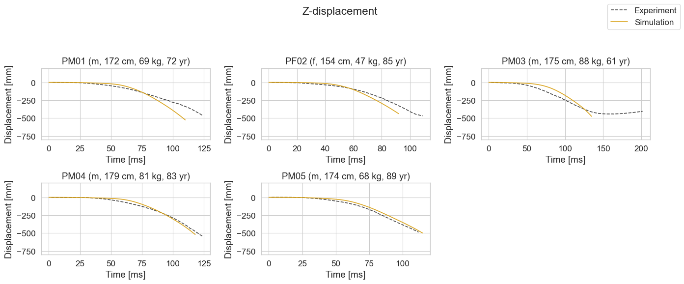
create_subplots(
figure_title = 'Z-displacement',
offset_exp_data_x = list(map(float, (hit_df['First leg contact [ms]'].tolist()))),
cut_sim_data = list(map(float, (hit_df['First head contact [ms]'].tolist()))),
sim_x_data = ('HEAD', 'z-displacement', 'time'),
sim_y_data = ('HEAD', 'z-displacement', 'displacement'),
exp_x_data = ('Head', 'time'),
exp_y_data = ('Head', 'z-displacement'),
sim_name1_legend = 'Simulation',
exp_name1_legend = 'Experiment',
x_label = 'Time [ms]',
y_label = 'Displacement [mm]',
x_lim = [0, 200],
y_lim = [-800, 200],
filename_save = 'results/figures/VIVA+_Paas_et_al_2015_z-displacement_time.svg'
)
Tibia and femur strains#
Show code cell source
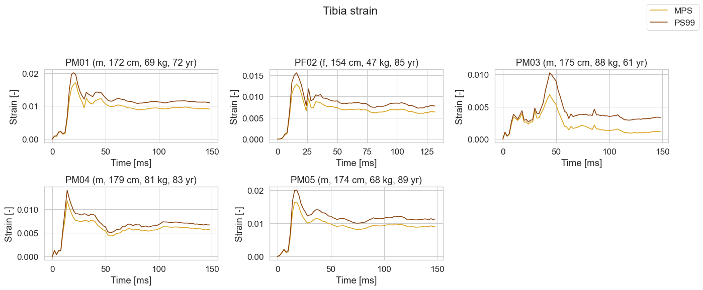
create_subplots(
figure_title = 'Tibia strain',
sim_x_data = ('BONES', 'Tibia_Cortical_R_PS99', 'time'),
sim_y_data = ('BONES', 'Tibia_Cortical_R_PS99', 'strain'),
sim_x_data2 = ('BONES', 'Tibia_Cortical_R_MPS', 'time'),
sim_y_data2 = ('BONES', 'Tibia_Cortical_R_MPS', 'strain'),
sim_name1_legend = 'MPS',
sim_name2_legend = 'PS99',
x_label = 'Time [ms]',
y_label = 'Strain [-]',
x_lim = [0, 200],
filename_save = 'results/figures/Paas_et_al_2015_tibia_r_strain_time.svg'
)
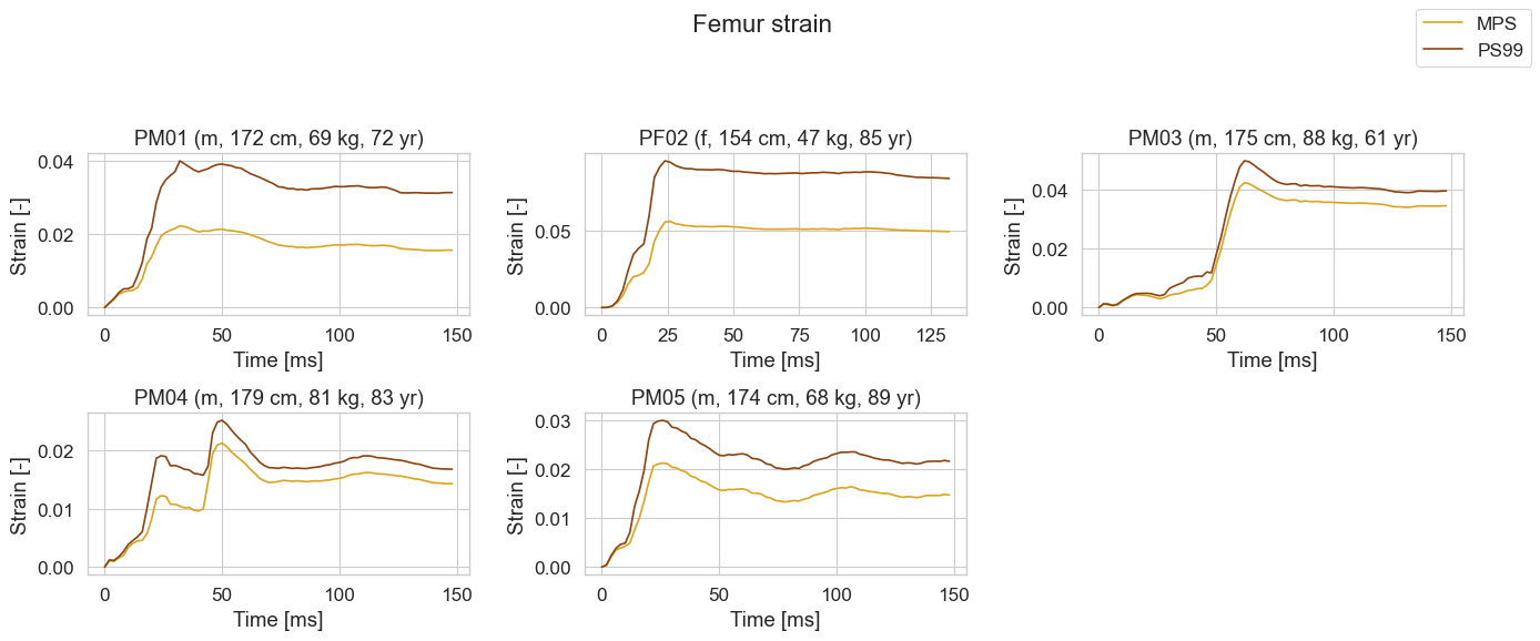
create_subplots(
figure_title = 'Femur strain',
sim_x_data = ('BONES', 'Femur_Cortical_R_PS99', 'time'),
sim_y_data = ('BONES', 'Femur_Cortical_R_PS99', 'strain'),
sim_x_data2 = ('BONES', 'Femur_Cortical_R_MPS', 'time'),
sim_y_data2 = ('BONES', 'Femur_Cortical_R_MPS', 'strain'),
sim_name1_legend = 'MPS',
sim_name2_legend = 'PS99',
x_label = 'Time [ms]',
y_label = 'Strain [-]',
x_lim = [0, 200],
filename_save = 'results/figures/Paas_et_al_2015_femur_r_strain_time.svg'
)
Energy time histories#
Show code cell source
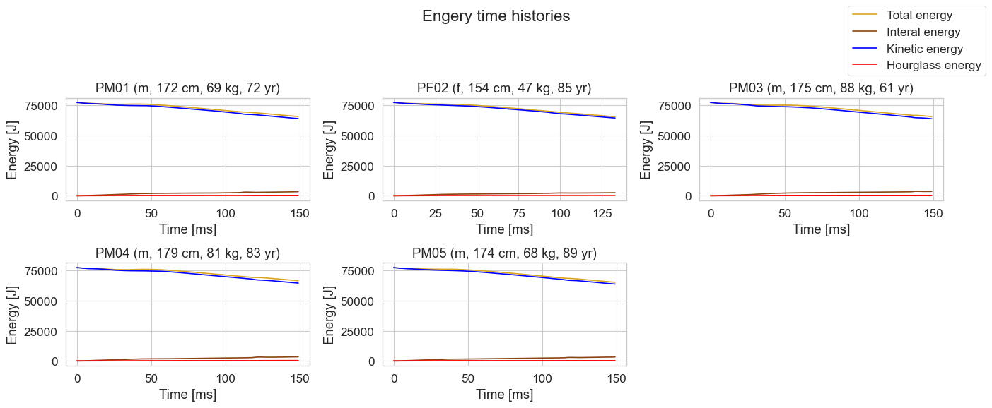
create_subplots(
figure_title = 'Engery time histories',
sim_x_data = ('MODEL', 'Total_Energy', 'time'),
sim_y_data = ('MODEL', 'Total_Energy', 'energy'),
sim_x_data2 = ('MODEL', 'Internal_Energy', 'time'),
sim_y_data2 = ('MODEL', 'Internal_Energy', 'energy'),
sim_x_data3 = ('MODEL', 'Kinetic_Energy', 'time'),
sim_y_data3 = ('MODEL', 'Kinetic_Energy', 'energy'),
sim_x_data4 = ('MODEL', 'Hourglass_Energy', 'time'),
sim_y_data4 = ('MODEL', 'Hourglass_Energy', 'energy'),
sim_name1_legend = 'Total energy',
sim_name2_legend = 'Interal energy',
sim_name3_legend = 'Kinetic energy',
sim_name4_legend = 'Hourglass energy',
x_label = 'Time [ms]',
y_label = 'Energy [J]',
x_lim = [0, 200],
filename_save = 'results/figures/Paas__interal_energy__kinetic_energy__time.svg'
)
Tibia and femur fracture risk#
Show code cell source
tibia_exp_fracture = ['no', 'yes', 'yes', 'yes', 'yes']
femur_exp_fracture = ['no', 'no', 'no', 'no', 'no']
tibia_PS99_peak_strain_array = find_peak_strains(
title = 'Tibia PS99 strain',
x_data = ('BONES', 'Tibia_Cortical_R_PS99', 'time'),
y_data = ('BONES', 'Tibia_Cortical_R_PS99', 'strain')
)
femur_PS99_peak_strain_array = find_peak_strains(
title = 'Femur PS99 strain',
x_data = ('BONES', 'Femur_Cortical_R_PS99', 'time'),
y_data = ('BONES', 'Femur_Cortical_R_PS99', 'strain')
)
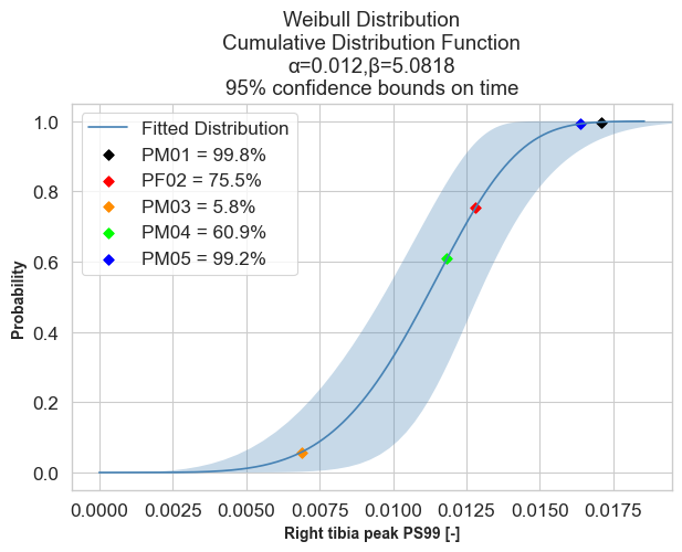
probability_list_tibia = plot_peak_strains_on_irc(
peak_strain_array = tibia_PS99_peak_strain_array,
x_label = 'Right tibia peak PS99 [-]',
filename_strains_irc = 'data/metadata/Tibia_injury-risk-curve/strains_tibia_for_IRC.csv'
)
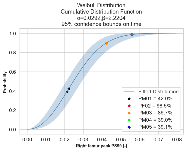
probability_list_femur = plot_peak_strains_on_irc(
peak_strain_array = femur_PS99_peak_strain_array,
x_label = 'Right femur peak PS99 [-]',
filename_strains_irc = 'data/metadata/Femur_injury-risk-curve/Schubert-2020_Femur_All-Strain-Curves-for-FRC.csv'
)
fracture_risks_df = pd.DataFrame({'Simulation': simulation_list,
'Tibia fracture probability [%]': probability_list_tibia,
'Experiment tibia fracture': np.array(tibia_exp_fracture),
'Femur fracture probability [%]': probability_list_femur,
'Experiment femur fracture': np.array(femur_exp_fracture),})
display(fracture_risks_df)
| Simulation | Tibia fracture probability [%] | Experiment tibia fracture | Femur fracture probability [%] | Experiment femur fracture | |
|---|---|---|---|---|---|
| 0 | PM01 | 99.7614 | no | 42.0278 | no |
| 1 | PF02 | 75.5104 | yes | 98.5391 | no |
| 2 | PM03 | 5.7665 | yes | 89.7069 | no |
| 3 | PM04 | 60.8827 | yes | 38.9985 | no |
| 4 | PM05 | 99.2236 | yes | 39.0745 | no |
ISO18571 objective rating for displacement-time histories#
Show code cell source
from objective_rating_metrics.rating import ISO18571
def calculate_iso_score(experiment_data_file, sim_x_data, sim_y_data, exp_x_data, exp_y_data, sim_data_for_calculation_y=None,):
    ratings = []
    for i in simulation_list:
        experimental_data = pd.read_csv(experiment_data_file, delimiter=';', header=[0,1,2,3], decimal='.')
        processed_data_path = os.path.join(processed_data_dir, i).replace('\\', '/')
        simData = pd.read_csv(os.path.join(processed_data_path, dynasaur_output_file_name),
                                    delimiter=';', na_values='-', header = [0,1,2,3])

        time_ref = np.array(experimental_data[(i,) + exp_x_data]).flatten()
        x_ref = np.array(experimental_data[(i,) + exp_y_data]).flatten()

        time_comp=np.array(simData[sim_x_data]).flatten()
        x_comp = simData[sim_y_data]

        if sim_data_for_calculation_y is not None:
            x_comp = x_comp + simData[sim_data_for_calculation_y]
        x_comp=np.array(x_comp).flatten()

        time_comp = np.delete(time_comp,np.s_[150:])
        x_comp = np.delete(x_comp, np.s_[150:])

        ind_nan = []
        ind_nan = np.where(np.isnan(x_ref))

        if len(ind_nan[0]) > 0:
            x_ref = x_ref[0:ind_nan[0][0]-1]
            x_time_ref = time_ref[0:ind_nan[0][0]-1]
            x_comp = x_comp[0:ind_nan[0][0]-1]
            x_time_comp = time_comp[0:ind_nan[0][0]-1]
        else:
            x_time_ref = time_ref
            x_time_comp = time_comp

        if len(x_ref) > len(x_comp):
            ind_end = len(x_comp)
            x_ref = x_ref[0:ind_end]
            x_time_ref = x_time_ref[0:ind_end]

        elif len(x_comp) > len(x_ref):
            ind_end = len(x_ref)
            x_comp = x_comp[0:ind_end]
            x_time_comp = x_time_comp[0:ind_end]

        ref = np.vstack((x_time_ref, x_ref)).T
        comp = np.vstack((x_time_comp, x_comp)).T

        iso_rating = ISO18571(reference_curve=ref, comparison_curve=comp)

        ratings.append([i,
        iso_rating.corridor_rating(),
        iso_rating.phase_rating(),
        iso_rating.magnitude_rating(),
        iso_rating.slope_rating(),
        iso_rating.overall_rating()])

    rating_array = []
    rating_array = np.append(rating_array, ratings)
    rating_array = rating_array.transpose()
    rating_array = np.reshape(rating_array, (5,6))

    return(rating_array)


# TODO implement time offset between test data and experiment


iso_ratings_x = calculate_iso_score(
sim_x_data = ('HEAD', 'x-displacement', 'time'),
sim_y_data = ('HEAD', 'x-displacement', 'displacement'),
experiment_data_file = 'data/experiment/Paas_et_al_2015_testdata.csv',
exp_x_data = ('Head', 'time'),
exp_y_data = ('Head', 'x-displacement'),
)

iso_ratings_x_df = pd.DataFrame(iso_ratings_x, columns=['Simulation', 'Corridor', 'Phase', 'Magnitude', 'Slope', 'Overall'])
print('ISO ratings for x-displacement')
display(iso_ratings_x_df)

iso_ratings_z = calculate_iso_score(
sim_x_data = ('HEAD', 'z-displacement', 'time'),
sim_y_data = ('HEAD', 'z-displacement', 'displacement'),
experiment_data_file = 'data/experiment/Paas_et_al_2015_testdata.csv',
exp_x_data = ('Head', 'time'),
exp_y_data = ('Head', 'z-displacement'),
)

iso_ratings_z_df = pd.DataFrame(iso_ratings_z, columns=['Simulation', 'Corridor', 'Phase', 'Magnitude', 'Slope', 'Overall'])
print('ISO ratings for z-displacement')
display(iso_ratings_z_df)
ISO ratings for x-displacement
| Simulation | Corridor | Phase | Magnitude | Slope | Overall | |
|---|---|---|---|---|---|---|
| 0 | PM01 | 0.305 | 0.752 | 0.007 | 0.643 | 0.403 |
| 1 | PF02 | 0.526 | 0.766 | 0.333 | 0.736 | 0.577 |
| 2 | PM03 | 0.607 | 0.533 | 0.661 | 0.536 | 0.589 |
| 3 | PM04 | 0.939 | 0.795 | 0.935 | 0.83 | 0.888 |
| 4 | PM05 | 0.824 | 0.636 | 0.918 | 0.833 | 0.807 |
ISO ratings for z-displacement
| Simulation | Corridor | Phase | Magnitude | Slope | Overall | |
|---|---|---|---|---|---|---|
| 0 | PM01 | 0.802 | 0.256 | 0.01 | 0.445 | 0.463 |
| 1 | PF02 | 0.885 | 0.86 | 0.933 | 0.823 | 0.877 |
| 2 | PM03 | 0.77 | 0.167 | 0.765 | 0.657 | 0.626 |
| 3 | PM04 | 0.973 | 0.139 | 0.228 | 0.606 | 0.584 |
| 4 | PM05 | 0.895 | 0.636 | 0.975 | 0.932 | 0.867 |