Pedestrian (Snedeker 2003)#
Model validation information
Performed by: Nico Erlinger
Reviewed by: Corina Klug
Added to VIVA+ Validation Catalog on 2022-11-30 by Corina Klug
Version |
Date |
Performed by |
LS-Dyna |
|---|---|---|---|
2022-11-30 |
Nico Erlinger |
9.3.1 |
|
0.3.2 |
2023-11-23 |
Corina Klug |
9.3.1 |
1.1.1 |
2024-05-22 |
Matej Kranjec |
12.2.1 |
© 2019-2024, OpenVT Organization (OVTO)
Available openly under under Creative Commons Attribution 4.0 International License 
References#
Experiments by Snedeker et al. (2003)#
Snedeker, J.G., Muser, M.H., Walz, F.H., 2003. Assessment of pelvis and upper leg injury risk in car-pedestrian collisions: comparison of accident statistics, impactor tests and a human body finite element model. Stapp Car Crash J 47, 437–457. References
Snedeker, J.G., Muser, M.H., Walz, F.H., 2003. Assessment of pelvis and upper leg injury risk in car-pedestrian collisions: comparison of accident statistics, impactor tests and a human body finite element model. Stapp Car Crash J 47, 437–457. Snedeker, J.G., Walz, F.H., Muser, M.H., Schroeder, G., Mueller, T.L., Müller, R., 2006. Microstructural insight into pedestrian pelvic fracture as assessed by high-resolution computed tomography. Journal of Biomechanics 39, 2709–2713. https://doi.org/10.1016/j.jbiomech.2005.09.008.
VIVA+ validation#
Manuscript currently under preparation
Information on the subjects/specimens#
PMHS |
Sex |
Height [cm] |
Weight [kg] |
Age [yr] |
Scale factor z (height) |
Scale factor xand y (weight) |
|---|---|---|---|---|---|---|
T1 |
f |
160 |
50 |
52 |
0.99 |
0.89 |
T2 |
f |
166 |
74 |
76 |
1.03 |
1.08 |
T3 |
m |
177 |
75 |
32 |
1.01 |
0.98 |
T4 |
m |
180 |
64 |
78 |
1.03 |
0.90 |
T5 |
m |
172 |
60 |
76 |
0.98 |
0.89 |
Loading and Boundary Conditions#
The vehicle shapes are differing in the different loadcases, which is shown exemplary for loadcase T1 & T5 in the figure below.

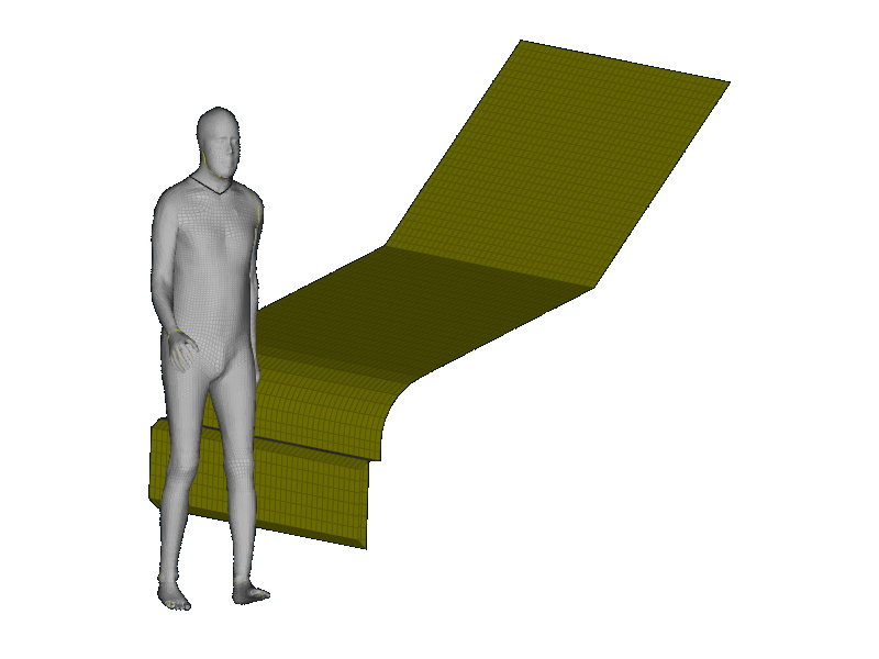
The initial velocity of the vehicle and its deceleration is prescribed. Open Issue: Implement damping to adress vehicle front oscillations (visible in energy plots).
Experimental responses#
The experimental responses from the original papers were digitalised.
Simulation metadata#
# Your name
name="Matej_Kranjec"

# LS-Dyna version (if you have not run the simulations on your own, fill in "example"):
dyna_executable_name="ls-dyna_mpp_s_R12.2.1_86_winx64_ifort170_msmpi"

# Overall number of CPUs
n_cpu = "40"

# Platform (from d3hsp file)
platform = "MS API x86_64"

# OS Level (from d3hsp file)
os_level = "Windows 11"

# Do not change! Date is filled in automatically
date = datetime.date.today().strftime("%Y-%m-%d")
# write metadata
metadata={
  "date": date,
  "name": name,
  "n_cpu": n_cpu,
  "dyna_executable_name": dyna_executable_name,
  "platform": platform,
  "os_level": os_level
}

with open(os.path.join(processed_data_dir, simulation_meta_file_name), 'w+') as f:
  json.dump(metadata, f, indent=4)
Results#
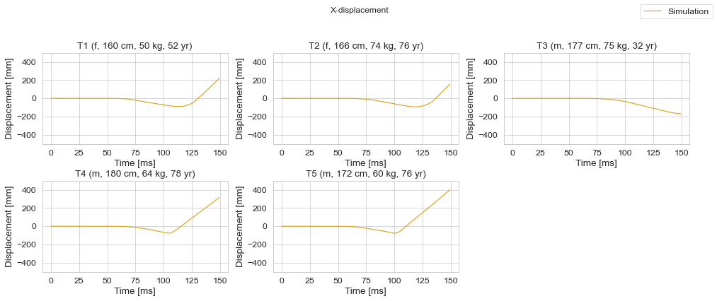
Trajectories#
Show code cell source
create_subplots(
figure_title = 'X-displacement',
sim_x_data = ('HEAD', 'x-displacement', 'time'),
sim_y_data = ('HEAD', 'x-displacement', 'displacement'),
sim_name1_legend = 'Simulation',
exp_name1_legend = 'Experiment',
x_label = 'Time [ms]',
y_label = 'Displacement [mm]',
x_lim = [0, 200],
y_lim = [-500, 500],
filename_save = 'results/figures/Snedeker_et_al_2003_x-displacement_time.svg'
)
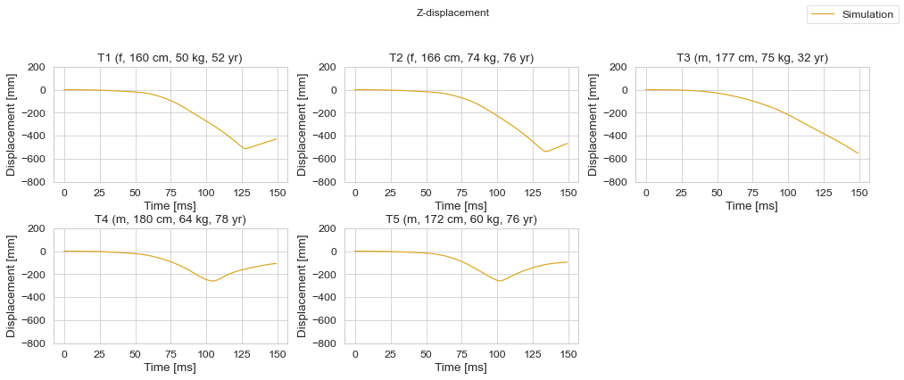
create_subplots(
figure_title = 'Z-displacement',
sim_x_data = ('HEAD', 'z-displacement', 'time'),
sim_y_data = ('HEAD', 'z-displacement', 'displacement'),
sim_name1_legend = 'Simulation',
exp_name1_legend = 'Experiment',
x_label = 'Time [ms]',
y_label = 'Displacement [mm]',
x_lim = [0, 200],
y_lim = [-800, 200],
filename_save = 'results/figures/Snedeker_et_al_2003_z-displacement_time.svg'
)
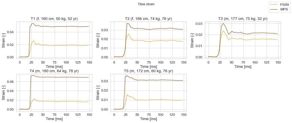
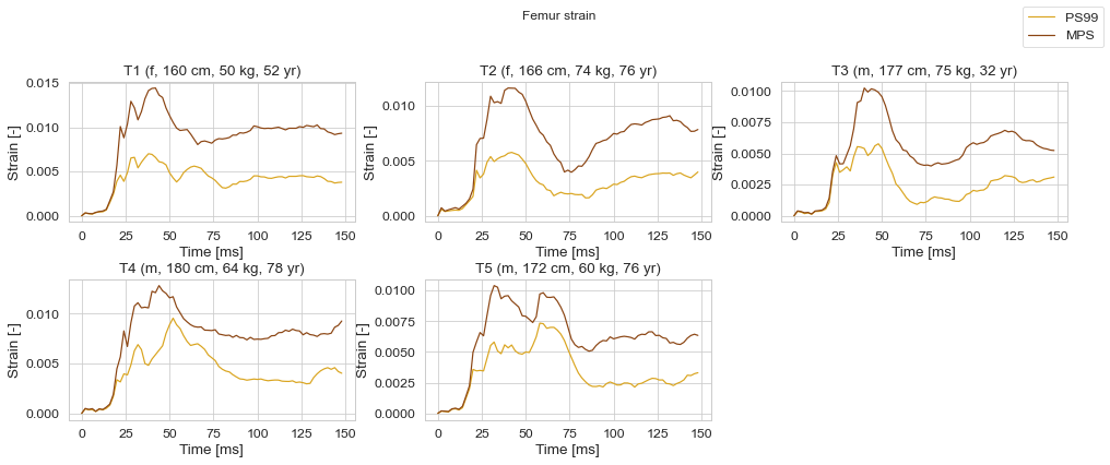
Femur and Tibia strains#
Show code cell source
create_subplots(
figure_title = 'Tibia strain',
sim_x_data = ('BONES', 'Tibia_Cortical_R_PS99', 'time'),
sim_y_data = ('BONES', 'Tibia_Cortical_R_PS99', 'strain'),
sim_x_data2 = ('BONES', 'Tibia_Cortical_R_MPS', 'time'),
sim_y_data2 = ('BONES', 'Tibia_Cortical_R_MPS', 'strain'),
sim_name1_legend = 'PS99',
sim_name2_legend = 'MPS',
x_label = 'Time [ms]',
y_label = 'Strain [-]',
x_lim = [0, 150],
filename_save = 'results/figures/Snedeker_et_al_2003_tibia_r_strain_time.svg'
)

create_subplots(
figure_title = 'Femur strain',
sim_x_data = ('BONES', 'Femur_Cortical_R_PS99', 'time'),
sim_y_data = ('BONES', 'Femur_Cortical_R_PS99', 'strain'),
sim_x_data2 = ('BONES', 'Femur_Cortical_R_MPS', 'time'),
sim_y_data2 = ('BONES', 'Femur_Cortical_R_MPS', 'strain'),
sim_name1_legend = 'PS99',
sim_name2_legend = 'MPS',
x_label = 'Time [ms]',
y_label = 'Strain [-]',
x_lim = [0, 150],
filename_save = 'results/figures/Snedeker_et_al_2003_femur_r_strain_time.svg'
)
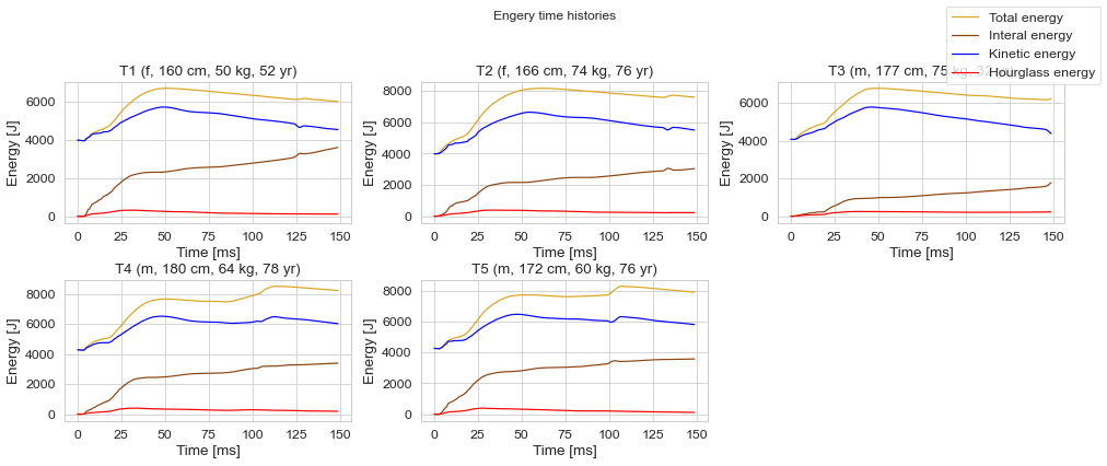
Energy time histories#
Show code cell source
create_subplots(
figure_title = 'Engery time histories',
sim_x_data = ('MODEL', 'Total_Energy', 'time'),
sim_y_data = ('MODEL', 'Total_Energy', 'energy'),
sim_x_data2 = ('MODEL', 'Internal_Energy', 'time'),
sim_y_data2 = ('MODEL', 'Internal_Energy', 'energy'),
sim_x_data3 = ('MODEL', 'Kinetic_Energy', 'time'),
sim_y_data3 = ('MODEL', 'Kinetic_Energy', 'energy'),
sim_x_data4 = ('MODEL', 'Hourglass_Energy', 'time'),
sim_y_data4 = ('MODEL', 'Hourglass_Energy', 'energy'),
sim_name1_legend = 'Total energy',
sim_name2_legend = 'Interal energy',
sim_name3_legend = 'Kinetic energy',
sim_name4_legend = 'Hourglass energy',
x_label = 'Time [ms]',
y_label = 'Energy [J]',
x_lim = [0, 150],
filename_save = 'results/figures/Snedeker_et_al_2003__interal_energy__kinetic_energy__time.svg'
)
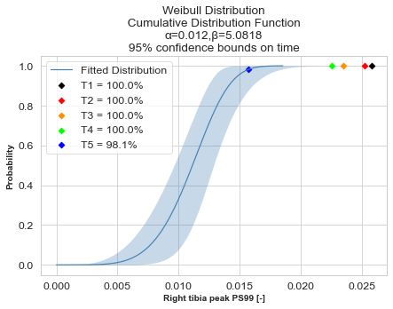
Plotting peak strains of tibia and femur on IRCs#
Show code cell source
def find_peak_strains(title, x_data, y_data):
    list = []
    for i in simulation_list:
        processed_data_path = os.path.join(processed_data_dir, i).replace('\\', '/')
        simData = pd.read_csv(os.path.join(processed_data_path, dynasaur_output_file_name),
                                    delimiter=';', na_values='-', header = [0,1,2,3])

        simData.fillna(0.0, inplace=True)
        sim_x_data = np.array(simData[x_data]).flatten()
        sim_y_data = np.array(simData[y_data]).flatten()

        peak_strain_ind = np.argmax(sim_y_data)
        peak_time = sim_x_data[peak_strain_ind]
        peak_strain = sim_y_data[peak_strain_ind]
        list.append([i, peak_time, peak_strain])

    list = np.reshape(list, (len(simulation_list), 3))
    return list

def plot_peak_strains_on_irc(x_label, filename_strains_irc, peak_strain_array):
    plotT1 = { "marker" :'D', "color" : 'black',}
    plotT2 = { "marker" :'D', "color" : 'red', }
    plotT3 = { "marker" :'D', "color" : 'darkorange',}
    plotT4 = { "marker" :'D', "color" : 'lime',}
    plotT5 = { "marker" :'D', "color" : 'blue',}

    sim_strain_data = peak_strain_array[:,2].astype(float)
    sim_name_data = peak_strain_array[:,0]
    df_strains_irc = pd.read_csv(filename_strains_irc, sep = ";")

    plt.figure(figsize=(7,5))
    weibull_fit = Fit_Weibull_2P(failures=list(df_strains_irc.PS99),show_probability_plot=False,print_results=False, CI=0.95, CI_type="time")

    weibull_fit.distribution.CDF(label='Fitted Distribution',color='steelblue')
    plt.xlabel(x_label, fontweight='semibold',fontsize=10)
    plt.ylabel("Probability",fontweight='semibold',fontsize=10)

    x_values = sim_strain_data.flatten()
    axs = plt.gca()
    line = axs.lines[0]
    IRC_distrib_x = line.get_xdata()
    IRC_distrib_y = line.get_ydata()

    probability_list = []
    for x in range(len(x_values)):
        smaller_values = np.where(IRC_distrib_x < x_values[x])
        bigger_values = np.where(IRC_distrib_x > x_values[x])

        ind_small = smaller_values[0][-1]
        ind_big = ind_small+1

        if ind_small == 199:
            y_value = 0.9999
        else:
            x_interp_array = [IRC_distrib_x[ind_small],IRC_distrib_x[ind_big]]
            y_interp_array = [IRC_distrib_y[ind_small],IRC_distrib_y[ind_big]]
            y_value = np.interp(x_values[x],x_interp_array,y_interp_array)

        simPlot = locals()["plot" + sim_name_data[x]]
        plt.scatter(x_values[x], y_value,**simPlot,label=sim_name_data[x] + ' = ' + str(round(y_value*100,1)) + '%')
        plt.legend(loc=0)
        probability_list.append(y_value*100)
    return(probability_list)
Show code cell source
tibia_exp_fracture = ['no', 'no', 'yes', 'yes', 'yes']
femur_exp_fracture = ['no', 'no', 'no', 'no', 'no']
tibia_PS99_peak_strain_array = find_peak_strains(
title = 'Tibia PS99 strain',
x_data = ('BONES', 'Tibia_Cortical_R_PS99', 'time'),
y_data = ('BONES', 'Tibia_Cortical_R_PS99', 'strain')
)
femur_PS99_peak_strain_array = find_peak_strains(
title = 'Femur PS99 strain',
x_data = ('BONES', 'Femur_Cortical_R_PS99', 'time'),
y_data = ('BONES', 'Femur_Cortical_R_PS99', 'strain')
)
probability_list_tibia = plot_peak_strains_on_irc(
peak_strain_array = tibia_PS99_peak_strain_array,
x_label = 'Right tibia peak PS99 [-]',
filename_strains_irc = 'data/metadata/Tibia_injury-risk-curve/strains_tibia_for_IRC.csv'
)
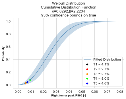
probability_list_femur = plot_peak_strains_on_irc(
peak_strain_array = femur_PS99_peak_strain_array,
x_label = 'Right femur peak PS99 [-]',
filename_strains_irc = 'data/metadata/Femur_injury-risk-curve/Schubert-2020_Femur_All-Strain-Curves-for-FRC.csv'
)
fracture_risks_df = pd.DataFrame({'Simulation': simulation_list,
'Tibia fracture probability [%]': probability_list_tibia,
'Experiment tibia fracture': np.array(tibia_exp_fracture),
'Femur fracture probability [%]': probability_list_femur,
'Experiment femur fracture': np.array(femur_exp_fracture),})
display(fracture_risks_df)
| Simulation | Tibia fracture probability [%] | Experiment tibia fracture | Femur fracture probability [%] | Experiment femur fracture | |
|---|---|---|---|---|---|
| 0 | T1 | 99.99 | no | 4.12596 | no |
| 1 | T2 | 99.99 | no | 2.69578 | no |
| 2 | T3 | 99.99 | yes | 2.70425 | no |
| 3 | T4 | 99.99 | yes | 8.0442 | no |
| 4 | T5 | 98.1308 | yes | 4.57149 | no |
Head impact times#
Show code cell source
hit_array=calculate_head_impact_time(
sim_x_data_leg = ('HBM', 'HBM_Leg_Vehicle_Contact_Transducer_x_force', 'time'),
sim_y_data_leg = ('HBM', 'HBM_Leg_Vehicle_Contact_Transducer_x_force', 'force'),
sim_x_data_head = ('HBM', 'HBM_Head_Vehicle_Contact_Transducer_z_force', 'time'),
sim_y_data_head = ('HBM', 'HBM_Head_Vehicle_Contact_Transducer_z_force', 'force')
)
hit_df = pd.DataFrame(hit_array, columns=['Simulation', 'First leg contact [ms]', 'First head contact [ms]', 'HIT [ms]'])
display(hit_df)
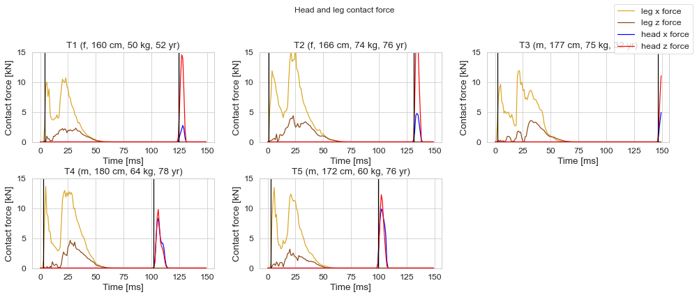
create_subplots(
figure_title = 'Head and leg contact force',
sim_x_data = ('HBM', 'HBM_Leg_Vehicle_Contact_Transducer_x_force', 'time'),
sim_y_data = ('HBM', 'HBM_Leg_Vehicle_Contact_Transducer_x_force', 'force'),
sim_x_data2 = ('HBM', 'HBM_Leg_Vehicle_Contact_Transducer_z_force', 'time'),
sim_y_data2 = ('HBM', 'HBM_Leg_Vehicle_Contact_Transducer_z_force', 'force'),
sim_x_data3 = ('HBM', 'HBM_Head_Vehicle_Contact_Transducer_x_force', 'time'),
sim_y_data3 = ('HBM', 'HBM_Head_Vehicle_Contact_Transducer_x_force', 'force'),
sim_x_data4 = ('HBM', 'HBM_Head_Vehicle_Contact_Transducer_z_force', 'time'),
sim_y_data4 = ('HBM', 'HBM_Head_Vehicle_Contact_Transducer_z_force', 'force'),
sim_name1_legend = 'leg x force',
sim_name2_legend = 'leg z force',
sim_name3_legend = 'head x force',
sim_name4_legend = 'head z force',
x_label = 'Time [ms]',
y_label = 'Contact force [kN]',
vertical_line1 = list(map(float, (hit_df['First leg contact [ms]'].tolist()))),
vertical_line2 = list(map(float, (hit_df['First head contact [ms]'].tolist()))),
x_lim = [0, 150],
y_lim = [0, 15],
)
| Simulation | First leg contact [ms] | First head contact [ms] | HIT [ms] | |
|---|---|---|---|---|
| 0 | T1 | 4.0 | 124.0 | 120 |
| 1 | T2 | 1.0 | 131.0 | 130 |
| 2 | T3 | 2.0 | 146.0 | 144 |
| 3 | T4 | 3.0 | 102.0 | 99 |
| 4 | T5 | 3.0 | 99.0 | 96 |