Single Rib (Forman 2020)#
Postprocessing of Single rib bending test based on Forman 2020
Version |
Date |
Performed by |
LS-Dyna |
|---|---|---|---|
0.3.2 |
2022-11-30 |
Johan Iraeus |
9.3.1 |
1.1.1 |
2024-05-22 |
Johan Iraeus |
12.2.1 |
Added to VIVA+ Validation Catalog on : 2022-11-30
© 2019-2023, OpenVT Organization (OVTO)
Available openly under Creative Commons Attribution 4.0 International License 
Experiment by Forman et al. (2020)#
Summary:#
The simulated data have previously been reported in:
Forman, J., “Small Female/Older Occupant Thoracic Biofidelity - Quasi-Static Rib Loading Report”, Report for NHTSA contract DTNH2215D000022/TO00001, Center for Applied Biomechanics, University of Virginia, March 2020

(Setup for the isolated VIVA+ 50F rib 6 model)
Experiment#
Information on the subjects/specimens#
Rib 6 and 7 from 10 female specimens (average age: 65 yrs, average mass: 44 kg, average height: 158 cm)
Loading and Boundary Conditions#
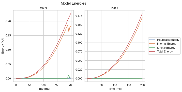
The ribs were loaded in a three point bending configuration, loading the ribs from the pleural to the cutaneous side. Distance between the 12mm diameter supports were 100 mm (112 mm center to center). The loading was applied with a 12mm diameter impactor at a quasi static loading speed of 2.54 mm/min. The loading speed in the simulation was increased to 0.0175 mm/ms, without observing any dynamic effects or kinetic energy.
Positioning#
The ribs were positioned according to the report, where it was stated that the samples were harvested between the posterior axillary and the midclavicular lines, roughly corresponding to the most lateral portion of the ribs.
Responses recorded#
The reference values from the paper were digitalised and are included in the package.
Other Notes for simulation#
As only female ribs were tested, only ribs from the 50F model is compared to the PMHS responses.
# Your name
name="Johan_Iraeus"

# LS-Dyna version (if you have not run the simulations on your own, fill in "example"):
dyna_executable_name="ls-dyna_mpp_s_R12_2_1_x64_centos79_ifort160_avx2_intelmpi-2018_sharelib"

# Overall number of CPUs
n_cpu = "32"

# Platform (from d3hsp file)
platform = "Intel-MPI 2018 Xeon64"

# OS Level (from d3hsp file)
os_level = "Linux CentOS 7.9 uom"

# Do not change! Date is filled in automatically
date = datetime.date.today().strftime("%Y-%m-%d")
# write metadata
metadata={
  "date": date,
  "name": name,
  "n_cpu": n_cpu,
  "dyna_executable_name": dyna_executable_name,
  "platform": platform,
  "os_level": os_level
}

with open(os.path.join(processed_data_dir, simulation_meta_file_name), 'w+') as f:
  json.dump(metadata, f, indent=4)
simData_R6
| impactor | MODEL | |||||||||||||
|---|---|---|---|---|---|---|---|---|---|---|---|---|---|---|
| displacement | force | Added_Mass | Total_Energy | Internal_Energy | Kinetic_Energy | Hourglass_Energy | ||||||||
| time | z_displacement | time | z_force | time | mass | time | energy | time | energy | time | energy | time | energy | |
| millisecond | dimensionless | millisecond | kilogram * millimeter / millisecond ** 2 | millisecond | kilogram | millisecond | kilogram * millimeter ** 2 / millisecond ** 2 | millisecond | kilogram * millimeter ** 2 / millisecond ** 2 | millisecond | kilogram * millimeter ** 2 / millisecond ** 2 | millisecond | kilogram * millimeter ** 2 / millisecond ** 2 | |
| 0 | 0.0 | 0.000000 | 0.000000 | -0.000002 | 0.0 | 0.0 | 0.0 | 6.399999e-19 | 0.0 | 6.399999e-19 | 0.0 | 0.000000e+00 | 0.0 | 0.000000e+00 |
| 1 | 2.0 | -0.000543 | 1.999997 | -0.000047 | 1.0 | 0.0 | 1.0 | 1.039815e-09 | 1.0 | 1.390605e-10 | 1.0 | 8.898066e-10 | 1.0 | 5.112739e-13 |
| 2 | 4.0 | -0.004016 | 3.999994 | -0.000127 | 2.0 | 0.0 | 2.0 | 1.771141e-08 | 2.0 | 3.104829e-09 | 2.0 | 1.414395e-08 | 2.0 | 6.638123e-12 |
| 3 | 6.0 | -0.012849 | 5.999991 | -0.000170 | 3.0 | 0.0 | 3.0 | 9.794863e-08 | 3.0 | 1.976291e-08 | 3.0 | 7.491285e-08 | 3.0 | 3.733480e-11 |
| 4 | 8.0 | -0.028533 | 7.999988 | -0.000180 | 4.0 | 0.0 | 4.0 | 3.397279e-07 | 4.0 | 6.244495e-08 | 4.0 | 2.662848e-07 | 4.0 | 1.004349e-10 |
| ... | ... | ... | ... | ... | ... | ... | ... | ... | ... | ... | ... | ... | ... | ... |
| 195 | NaN | NaN | NaN | NaN | 195.0 | 0.0 | 195.0 | 2.182959e-01 | 195.0 | 1.769010e-01 | 195.0 | 1.405519e-03 | 195.0 | 3.325664e-04 |
| 196 | NaN | NaN | NaN | NaN | 196.0 | 0.0 | 196.0 | 2.203564e-01 | 196.0 | 1.804041e-01 | 196.0 | 1.243476e-03 | 196.0 | 3.572257e-04 |
| 197 | NaN | NaN | NaN | NaN | 197.0 | 0.0 | 197.0 | 2.225613e-01 | 197.0 | 1.801528e-01 | 197.0 | 1.493712e-03 | 197.0 | 3.490976e-04 |
| 198 | NaN | NaN | NaN | NaN | 198.0 | 0.0 | 198.0 | 2.247371e-01 | 198.0 | 1.796059e-01 | 198.0 | 1.940289e-03 | 198.0 | 3.217213e-04 |
| 199 | NaN | NaN | NaN | NaN | 199.0 | 0.0 | 199.0 | 2.267868e-01 | 199.0 | 1.829345e-01 | 199.0 | 6.433512e-04 | 199.0 | 3.157631e-04 |
200 rows × 14 columns
Show code cell source
fig_energy, (ax1,ax2) = plt.subplots(nrows=1, ncols=2, figsize=(8,5))
fig_energy.suptitle('Model Energies')
#plt.set_title('Simulation #1')
#plt.set_ylabel('Energies (J)')
ax1.plot(simData_R6.MODEL.Hourglass_Energy.time, simData_R6.MODEL.Hourglass_Energy.energy, label = "Hourglass Energy")
ax1.plot(simData_R6.MODEL.Internal_Energy.time, simData_R6.MODEL.Internal_Energy.energy, label = "Internal Energy")
ax1.plot(simData_R6.MODEL.Kinetic_Energy.time, simData_R6.MODEL.Kinetic_Energy.energy, label = "Kinetic Energy")
ax1.plot(simData_R6.MODEL.Total_Energy.time, simData_R6.MODEL.Total_Energy.energy, label = "Total Energy")

ax2.plot(simData_R7.MODEL.Hourglass_Energy.time, simData_R7.MODEL.Hourglass_Energy.energy)
ax2.plot(simData_R7.MODEL.Internal_Energy.time, simData_R7.MODEL.Internal_Energy.energy)
ax2.plot(simData_R7.MODEL.Kinetic_Energy.time, simData_R7.MODEL.Kinetic_Energy.energy)
ax2.plot(simData_R7.MODEL.Total_Energy.time, simData_R7.MODEL.Total_Energy.energy)

ax1.set(xlabel="Time [ms]", ylabel="Energy [kJ]", title = 'Rib 6')
ax2.set(xlabel="Time [ms]", title = 'Rib 7')

fig_energy.legend(loc='center left', bbox_to_anchor=(1, 0.5))
fig_energy.tight_layout(pad=0.5)
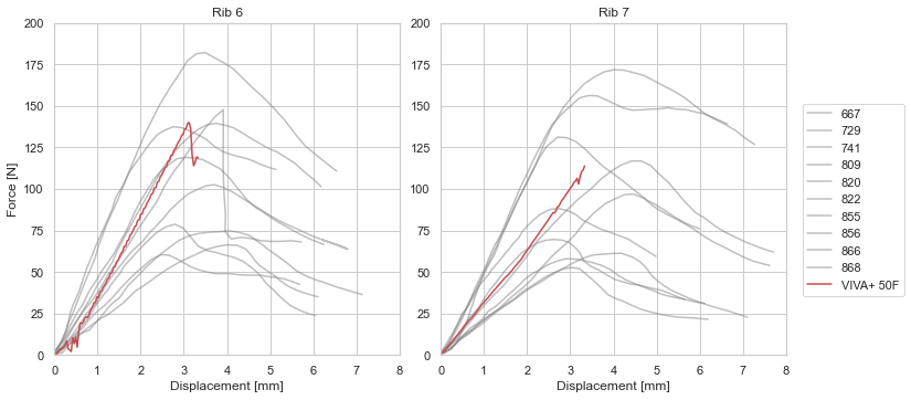
Force-Deflection Plots#
The figures below compares the predicted force-deflection based on the 50F with the PMHS responses. The jump in force is when the impactor contact slips over the rib.
Show code cell source
fig, (ax1, ax2) = plt.subplots(nrows=1, ncols=2, figsize= (10,5))

for col in range(0,19,2):
    ax1.plot(exp_rib_6.iloc[:,col], exp_rib_6.iloc[:,col+1], label = exp_rib_6.columns[col].split('_')[-2],**plotExperiment)

for col in range(0,19,2):
    ax2.plot(exp_rib_7.iloc[:,col], exp_rib_7.iloc[:,col+1], **plotExperiment)

ax1.plot(simData_R6.impactor.displacement.z_displacement*(-1), simData_R6.impactor.force.z_force*(-1000), label = 'VIVA+ 50F',**plot50F) # (-1 ) for positive dz and (-1000) from KN to N
ax2.plot(simData_R7.impactor.displacement.z_displacement *(-1), simData_R7.impactor.force.z_force*(-1000), **plot50F)

ax1.set(xlabel="Displacement [mm]", ylabel="Force [N]", title = 'Rib 6', xlim =(0,8), ylim =(0,200))
ax2.set(xlabel="Displacement [mm]", title = 'Rib 7', xlim =(0,8),  ylim =(0,200))

fig.legend(loc='center left', bbox_to_anchor=(1, 0.5))
fig.tight_layout(pad=0.5)
plt.show()