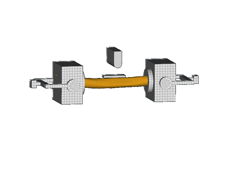
Femur shaft (Ivarsson 2009)#
Validation model information#
Postprocessing of femur shaft validations based on Ivarsson et al. 2009
Performed by: Nico Erlinger
Reviewed by: Corina Klug Added to VIVA+ Validation Catalog on: 2022-10-21
Version |
Date |
Performed by |
LS-Dyna |
|---|---|---|---|
0.3.2 |
2022-10-19 |
Nico Erlinger |
9.3.1 |
1.1.0 |
2024-05-22 |
Corina Klug |
9.3.1 |
© 2019-2024, OpenVT Organization (OVTO)
The Jupyter notebooks are licensed under Creative Commons Attribution 4.0 International License 
Reference#
A. Schubert, N. Erlinger, C. Leo, J. Iraeus, J. John, C. Klug (2021): “Development of a 50th Percentile Female Femur Model”, IRCOBI conference proceedings, http://www.ircobi.org/wordpress/downloads/irc21/pdf-files/2138.pdf
Experiments by Ivarsson et al. (2009)#
Ivarsson, B. J.; Genovese, D.; Crandall, J. R.; Bolton, J. R.; Untaroiu, C. D.; Bose, D. The Tolerance of the Femoral Shaft in Combined Axial Compression and Bending Loading in Stapp Car Crash Journal, Vol. 53, 2009.
Summary#
In total 42 tests of femur shaft were replicated by prescribing the vertical motion to the impactor (approx. 1.5 m/s). In addition, an axial force (approx. 4, 8, 12 or 16 kN) was applied for combined tests (axial compression and three-point bending).
Information on the subjects/specimens
Female specimens (n=16) are listed on the left side and male specimens (n=23) on the right side.
Specimen |
Loading type |
Loading direction |
Side |
Donor age |
|---|---|---|---|---|
1.18 |
co |
AP |
L |
64 |
1.19 |
co |
PA |
R |
64 |
1.20 |
co |
PA |
L |
40 |
1.21 |
co |
AP |
R |
40 |
1.22 |
co |
AP |
L |
45 |
1.23 |
co |
AP |
R |
45 |
1.24 |
co |
AP |
L |
60 |
1.26 |
co |
AP |
L |
50 |
1.27 |
co |
AP |
R |
50 |
1.28 |
co |
AP |
L |
56 |
1.29* |
co |
PA |
R |
56 |
1.32 |
be |
PA |
L |
52 |
1.33 |
be |
AP |
R |
52 |
1.35 |
be |
PA |
L |
62 |
1.36 |
be |
PA |
R |
62 |
2.10 |
be |
AP |
L |
57 |
1.01 |
co |
PA |
L |
51 |
1.02 |
co |
PA |
R |
51 |
1.03 |
co |
PA |
L |
62 |
1.04 |
co |
PA |
R |
62 |
1.05 |
co |
AP |
L |
62 |
1.06 |
co |
PA |
R |
62 |
1.07 |
co |
PA |
L |
49 |
1.08 |
co |
AP |
R |
49 |
1.09 |
co |
AP |
R |
62 |
1.10 |
co |
PA |
L |
44 |
1.11 |
co |
PA |
R |
44 |
1.12 |
co |
AP |
L |
58 |
1.13 |
co |
AP |
R |
58 |
1.14 |
co |
AP |
L |
65 |
1.15 |
co |
PA |
R |
65 |
1.16 |
co |
AP |
L |
53 |
1.17 |
co |
AP |
R |
53 |
1.30 |
co |
PA |
L |
62 |
1.34 |
be |
AP |
R |
63 |
1.37 |
be |
AP |
L |
45 |
1.38 |
be |
PA |
R |
45 |
2.06 |
be |
AP |
L |
39 |
2.07b |
be |
PA |
R |
51 |
Abbreviations: |
co : combined (axial compression and three-point bending
be : three-point bending (no axial compression)
L : left side
R : right side
AP : anterior-posterior
PA : posterior-anterior
Loading and Boundary Conditions#
The displacement-time histories from the diagrams published by Ivarsson et al. (2009) were digitised with WebPlotDigitizer v4.4 (https://automeris.io/WebPlotDigitizer).
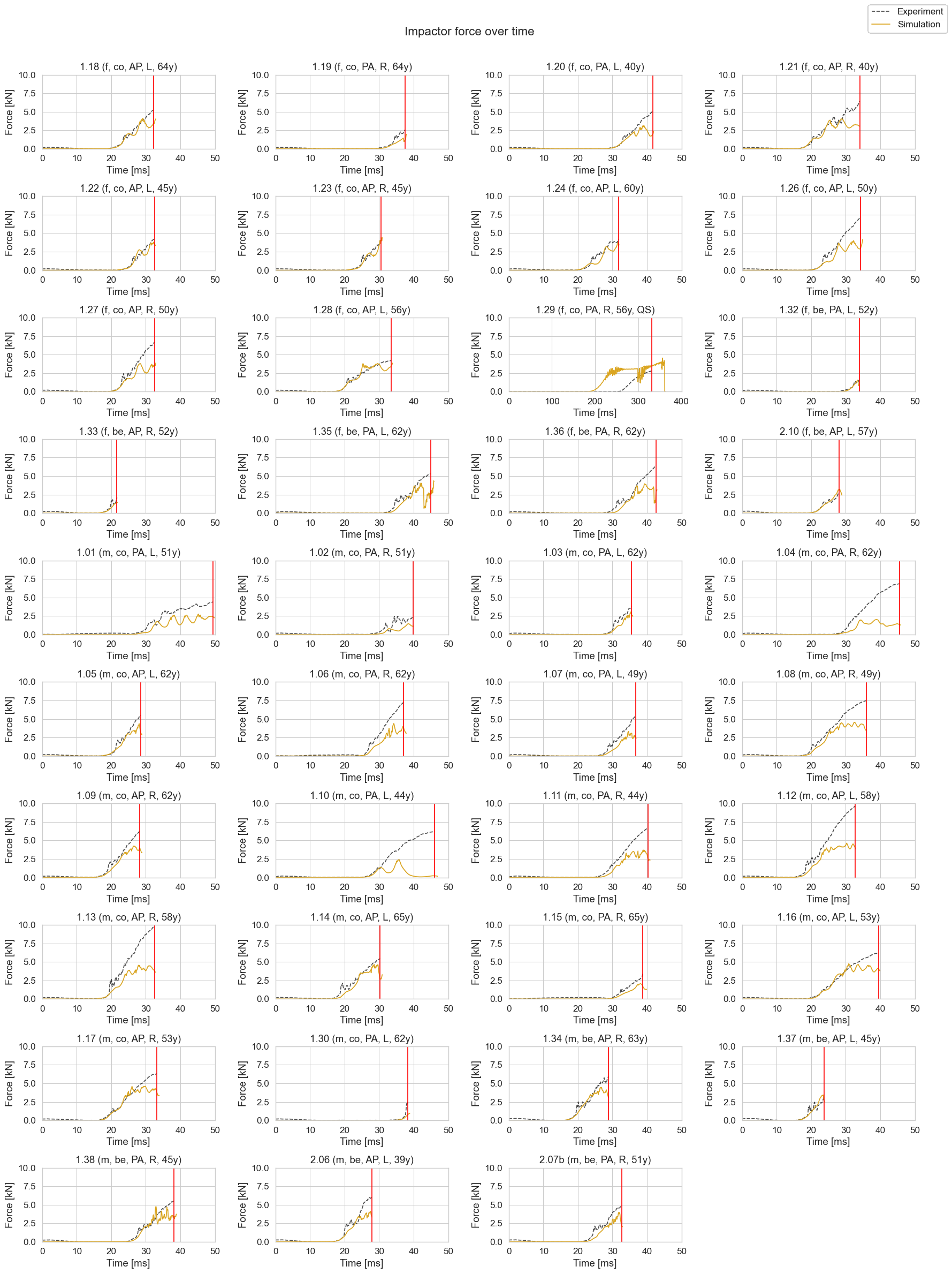
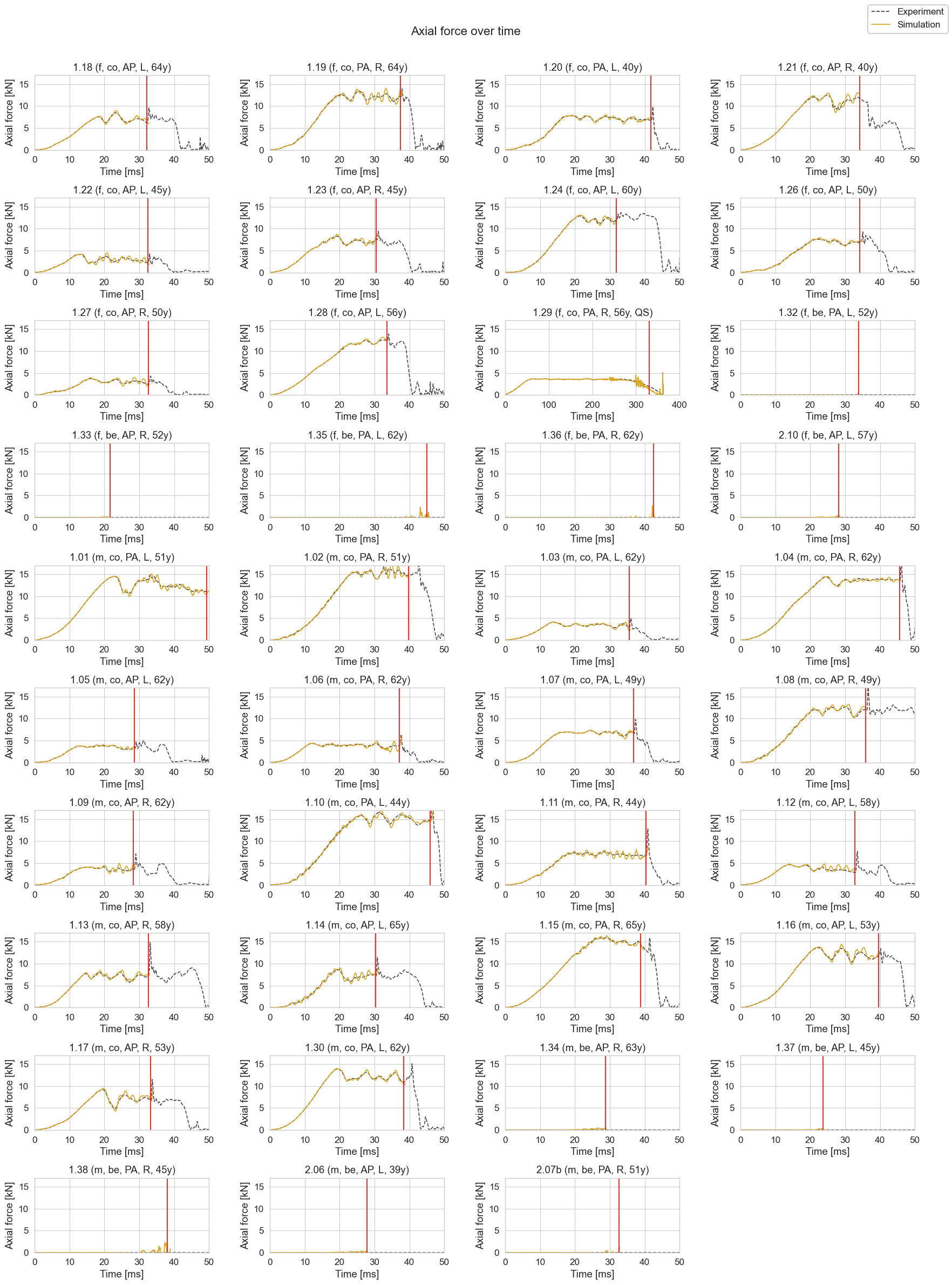
Experimental responses#
The force-time curves of the impactor and the axial loadcell were downloaded from the NHTSA Biomchanics Test Database (www.nhtsa.gov/research-data/research-testing-databases).
Show code cell content
simulation_list = ['1_18', '1_19', '1_20', '1_21', '1_22', '1_23', '1_24', '1_26', '1_27', '1_28',
                   '1_29', '1_32', '1_33', '1_35', '1_36', '2_10', '1_01', '1_02', '1_03', '1_04',
                   '1_05', '1_06', '1_07', '1_08', '1_09', '1_10', '1_11', '1_12', '1_13', '1_14',
                   '1_15', '1_16', '1_17', '1_30', '1_34', '1_37', '1_38', '2_06', '2_07b']

date = datetime.date.today().strftime('%Y-%m-%d')
dynasaur_output_file_name = 'Dynasaur_output.csv'
processed_data_dir = f'data/processed/{date}'
#processed_data_dir=f'data/processed/240522'
Results#
Show code cell source
simulation_list = ['1_18', '1_19', '1_20', '1_21', '1_22', '1_23', '1_24', '1_26', '1_27', '1_28',
'1_29', '1_32', '1_33', '1_35', '1_36', '2_10', '1_01', '1_02', '1_03', '1_04',
'1_05', '1_06', '1_07', '1_08', '1_09', '1_10', '1_11', '1_12', '1_13', '1_14',
'1_15', '1_16', '1_17', '1_30', '1_34', '1_37', '1_38', '2_06', '2_07b']
simulation_titles = ['1.18 (f, co, AP, L, 64y)',
'1.19 (f, co, PA, R, 64y)',
'1.20 (f, co, PA, L, 40y)',
'1.21 (f, co, AP, R, 40y)',
'1.22 (f, co, AP, L, 45y)',
'1.23 (f, co, AP, R, 45y)',
'1.24 (f, co, AP, L, 60y)',
'1.26 (f, co, AP, L, 50y)',
'1.27 (f, co, AP, R, 50y)',
'1.28 (f, co, AP, L, 56y)',
'1.29 (f, co, PA, R, 56y, QS)',
'1.32 (f, be, PA, L, 52y)',
'1.33 (f, be, AP, R, 52y)',
'1.35 (f, be, PA, L, 62y)',
'1.36 (f, be, PA, R, 62y)',
'2.10 (f, be, AP, L, 57y)',
'1.01 (m, co, PA, L, 51y)',
'1.02 (m, co, PA, R, 51y)',
'1.03 (m, co, PA, L, 62y)',
'1.04 (m, co, PA, R, 62y)',
'1.05 (m, co, AP, L, 62y)',
'1.06 (m, co, PA, R, 62y)',
'1.07 (m, co, PA, L, 49y)',
'1.08 (m, co, AP, R, 49y)',
'1.09 (m, co, AP, R, 62y)',
'1.10 (m, co, PA, L, 44y)',
'1.11 (m, co, PA, R, 44y)',
'1.12 (m, co, AP, L, 58y)',
'1.13 (m, co, AP, R, 58y)',
'1.14 (m, co, AP, L, 65y)',
'1.15 (m, co, PA, R, 65y)',
'1.16 (m, co, AP, L, 53y)',
'1.17 (m, co, AP, R, 53y)',
'1.30 (m, co, PA, L, 62y)',
'1.34 (m, be, AP, R, 63y)',
'1.37 (m, be, AP, L, 45y)',
'1.38 (m, be, PA, R, 45y)',
'2.06 (m, be, AP, L, 39y)',
'2.07b (m, be, PA, R, 51y)']
time_for_strain_eval = [32.2, 37.5, 41.7, 34.1, 32.5, 30.5, 31.8, 34.2, 32.6, 33.5, 330.7, 33.9, 21.6, 45,
42.6, 28.1, 49.4, 39.8, 35.5, 45.6, 28.6, 37.1, 36.8, 35.9, 28.3, 46, 40.3, 32.8,
32.6, 30.3, 38.8, 39.6, 33.2, 38.3, 28.8, 23.7, 38.1, 27.9, 32.7]
experiment_data_dir = 'data/experiment/'
#processed_data_dir = f'data/processed/{date}_{name}'
#processed_data_dir = f'data/processed/2022-10-19_Name_of_person'
def create_subplots(experiment_file, figure_title, sim_x_data, sim_y_data, sim_x_data2, sim_y_data2,
sim_name1_legend, sim_name2_legend, x_label, y_label, x_lim, y_lim, sign_swap_exp_data,
sign_swap_sim_data, filename_save):
figure, ((ax1, ax2, ax3, ax4), (ax5, ax6, ax7, ax8), (ax9, ax10, ax11, ax12), (ax13, ax14, ax15, ax16),
(ax17, ax18, ax19, ax20), (ax21, ax22, ax23, ax24), (ax25, ax26, ax27, ax28), (ax29, ax30, ax31, ax32),
(ax33, ax34, ax35, ax36), (ax37, ax38, ax39, ax40)) = plt.subplots(10,4, figsize=(18,24))
axs = [ax1, ax2, ax3, ax4, ax5, ax6, ax7, ax8, ax9, ax10, ax11, ax12, ax13, ax14, ax15, ax16, ax17, ax18, ax19,
ax20, ax21, ax22, ax23, ax24, ax25, ax26, ax27, ax28, ax29, ax30, ax31, ax32, ax33, ax34, ax35, ax36,
ax37, ax38, ax39, ax40]
figure.suptitle(figure_title)
figure.delaxes(axs[39])
figure.tight_layout(pad=3)
if experiment_file is not None:
experimental_data = pd.read_csv(experiment_data_dir + experiment_file, delimiter=';', header=[0], decimal='.')
plot_style_experimental = {"linestyle" :'--', "color" : 'black', "alpha" : 0.7}
plot_style_simulation = {"linestyle" :'-', "color" : 'goldenrod'}
plot_style_simulation2 = {"linestyle" :'-', "color" : 'saddlebrown'}
counter = 0
for i in simulation_list:
if experiment_file is not None:
x_data = experimental_data['Time'].values
y_data = experimental_data[i].values * sign_swap_exp_data
y_data = experimental_data[i].values
axs[counter].plot(x_data, y_data, **plot_style_experimental)
figure.legend(('Experiment', 'Simulation'), loc='upper right')
processed_data_path = os.path.join(processed_data_dir, i).replace('\\', '/')
simData = pd.read_csv(os.path.join(processed_data_path, dynasaur_output_file_name),
delimiter=';', na_values='-', header = [0,1,2,3])
x_data = simData[sim_x_data]
y_data = simData[sim_y_data]
y_data = y_data * sign_swap_sim_data
axs[counter].plot(x_data, y_data, **plot_style_simulation)
if sim_x_data2 and sim_x_data2 is not None:
x_data = simData[sim_x_data2]
y_data = simData[sim_y_data2]
y_data = y_data * sign_swap_sim_data
axs[counter].plot(x_data, y_data, **plot_style_simulation2)
figure.legend((sim_name1_legend, sim_name2_legend), loc='upper right')
axs[counter].set(xlabel=x_label)
axs[counter].set_ylabel(y_label)
if i is not '1_29':
axs[counter].set_xlim(x_lim)
else:
axs[counter].set_xlim(0, 400)
axs[counter].set_ylim(y_lim)
axs[counter].title.set_text(simulation_titles[counter])
axs[counter].axvline(x=time_for_strain_eval[counter], color='red')
counter += 1
figure.savefig(filename_save, format='svg', bbox_inches='tight')
figure_title = 'Impactor force over time'
experiment_file = 'Ivarsson_et_al_2009_impactor_force.csv'
sim_x_data = 'FEMUR', 'Impactor_rcforc_z', 'time'
sim_y_data = 'FEMUR', 'Impactor_rcforc_z', 'force'
sim_x_data2 = None
sim_y_data2 = None
sim_name1_legend = None
sim_name2_legend = None
x_label = 'Time [ms]'
y_label = 'Force [kN]'
x_lim = [0, 50]
y_lim = [0, 10]
sign_swap_exp_data = 1
sign_swap_sim_data = 1
filename_save = 'results/figures/VIVA+_Ivarsson_et_al_2009_impactor_force_time.svg'
create_subplots(experiment_file, figure_title, sim_x_data, sim_y_data, sim_x_data2, sim_y_data2, sim_name1_legend,
sim_name2_legend, x_label, y_label, x_lim, y_lim, sign_swap_exp_data, sign_swap_sim_data, filename_save)
figure_title = 'Axial force over time'
experiment_file = 'Ivarsson_et_al_2009_axial_force.csv'
sim_x_data = 'FEMUR', 'Axial_secforc_x', 'time'
sim_y_data = 'FEMUR', 'Axial_secforc_x', 'force'
sim_x_data2 = None
sim_y_data2 = None
sim_name1_legend = None
sim_name2_legend = None
x_label = 'Time [ms]'
y_label = 'Axial force [kN]'
x_lim = [0, 50]
y_lim = [0, 17]
sign_swap_exp_data = 1
sign_swap_sim_data = 1
filename_save = 'results/figures/Ivarsson_et_al_2009_axial_force_time.svg'
create_subplots(experiment_file, figure_title, sim_x_data, sim_y_data, sim_x_data2, sim_y_data2, sim_name1_legend,
sim_name2_legend, x_label, y_label, x_lim, y_lim, sign_swap_exp_data, sign_swap_sim_data, filename_save)
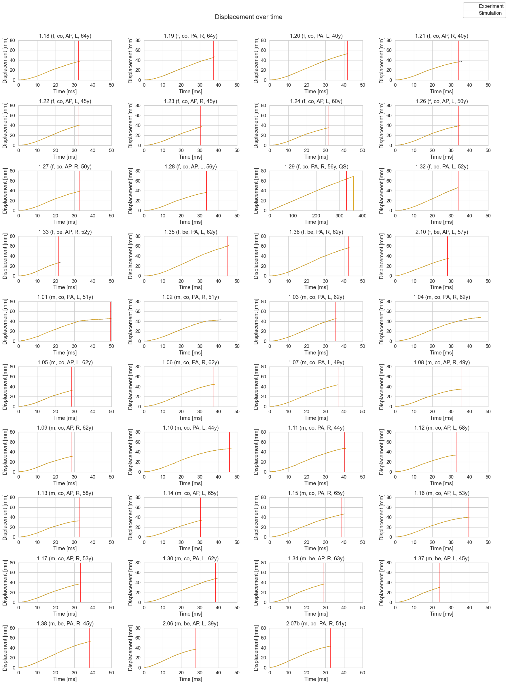
figure_title = 'Displacement over time'
experiment_file = 'Ivarsson_et_al_2009_impactor_displacement.csv'
sim_x_data = 'FEMUR', 'Impactor_nodout_z', 'time'
sim_y_data = 'FEMUR', 'Impactor_nodout_z', 'displacement'
sim_x_data2 = None
sim_y_data2 = None
sim_name1_legend = None
sim_name2_legend = None
x_label = 'Time [ms]'
y_label = 'Displacement [mm]'
x_lim = [0, 50]
y_lim = [0, 80]
sign_swap_exp_data = 1
sign_swap_sim_data = -1
filename_save = 'results/figures/Ivarsson_et_al_2009_displacement_time.svg'
create_subplots(experiment_file, figure_title, sim_x_data, sim_y_data, sim_x_data2, sim_y_data2, sim_name1_legend,
sim_name2_legend, x_label, y_label, x_lim, y_lim, sign_swap_exp_data, sign_swap_sim_data, filename_save)
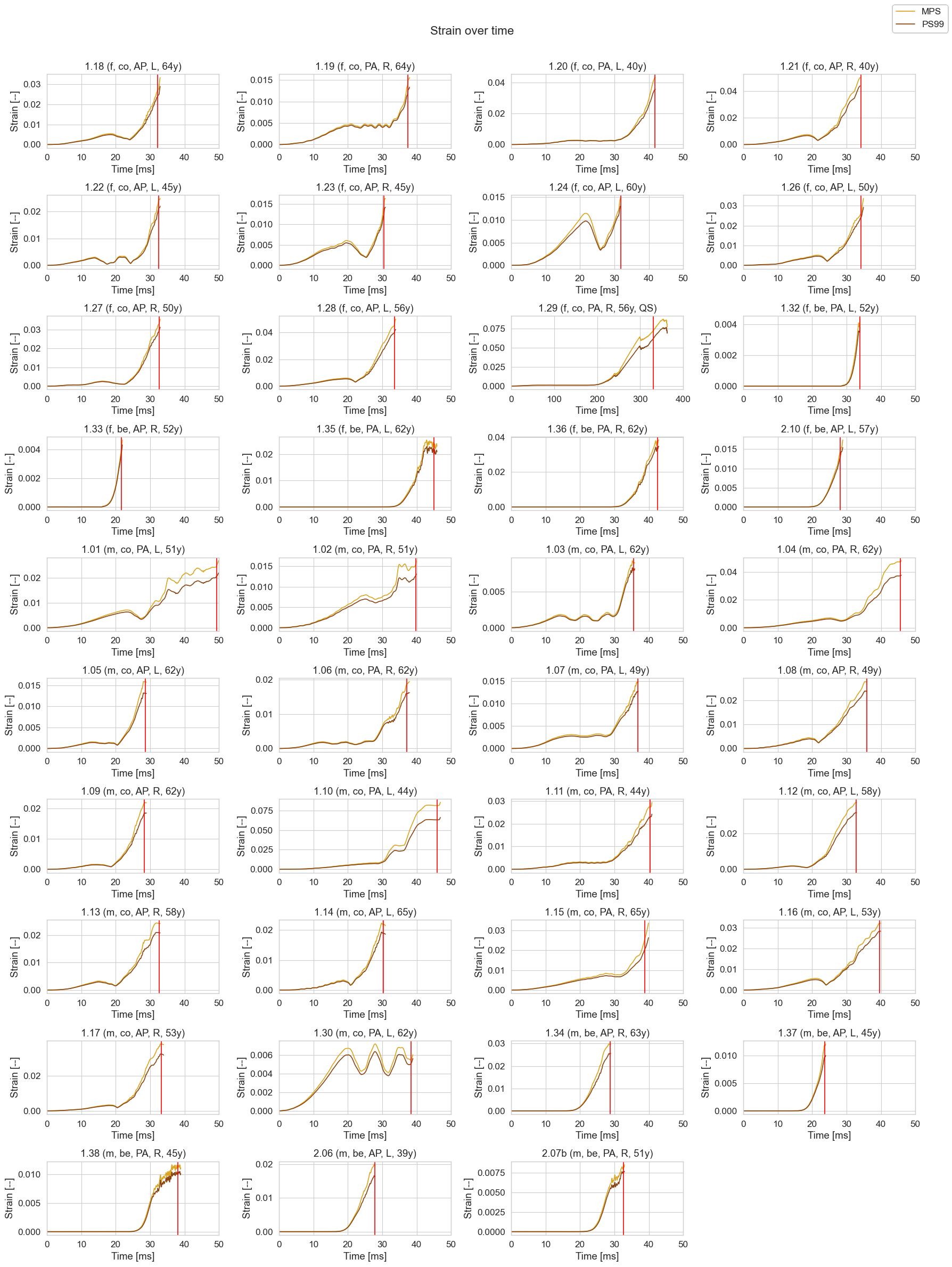
figure_title = 'Strain over time'
experiment_file = None
sim_x_data = 'BONES', 'Femur_Cortical_L_MPS_history', 'time'
sim_y_data = 'BONES', 'Femur_Cortical_L_MPS_history', 'strain'
sim_x_data2 = 'BONES', 'Femur_Cortical_L_PS99_history', 'time'
sim_y_data2 = 'BONES', 'Femur_Cortical_L_PS99_history', 'strain'
sim_name1_legend = 'MPS'
sim_name2_legend = 'PS99'
x_label = 'Time [ms]'
y_label = 'Strain [--]'
x_lim = [0, 50]
y_lim = None
sign_swap_exp_data = 1
sign_swap_sim_data = 1
filename_save = 'results/figures/Ivarsson_et_al_2009_strain_time.svg'
create_subplots(experiment_file, figure_title, sim_x_data, sim_y_data, sim_x_data2, sim_y_data2, sim_name1_legend,
sim_name2_legend, x_label, y_label, x_lim, y_lim, sign_swap_exp_data, sign_swap_sim_data, filename_save)
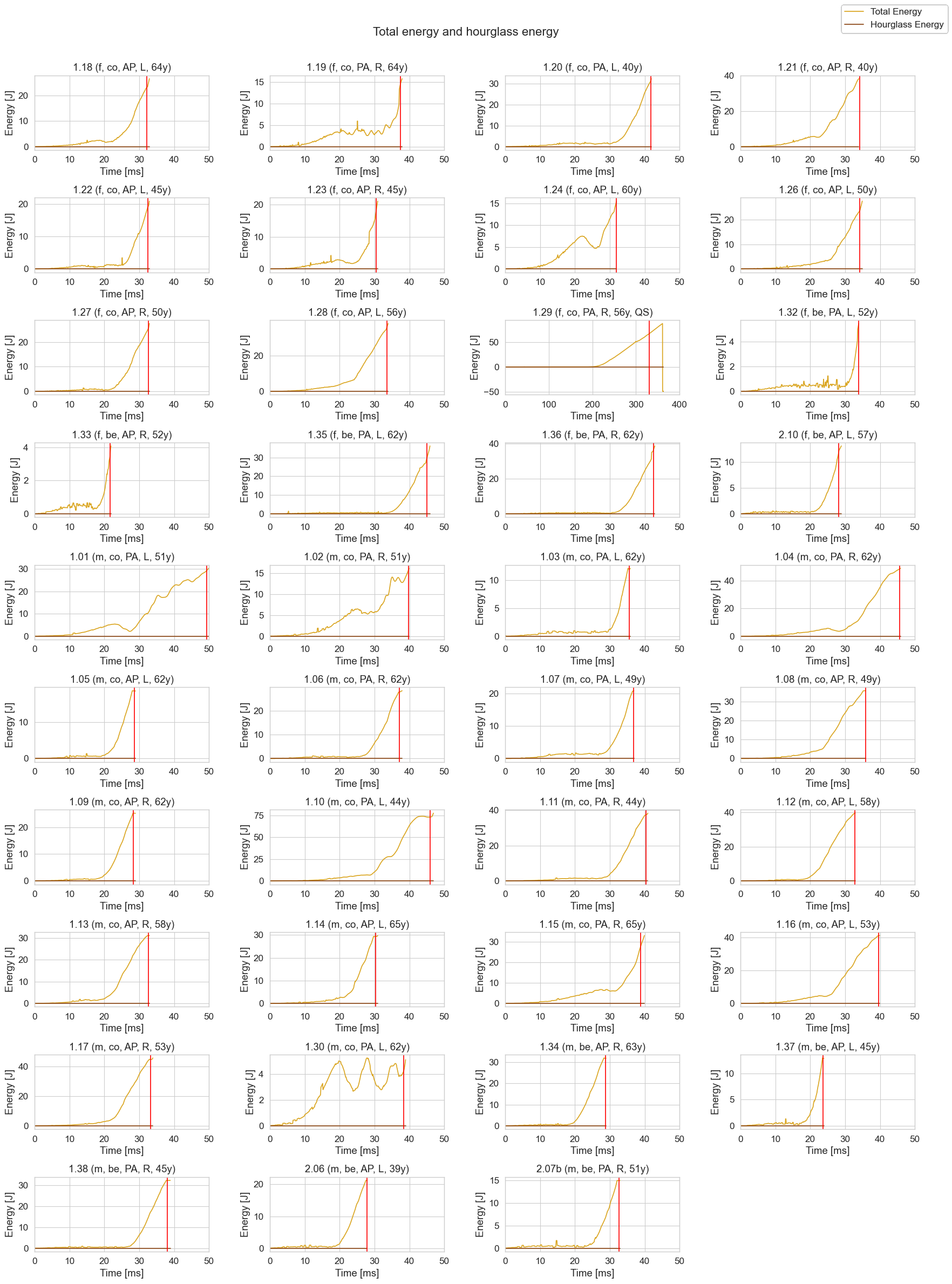
figure_title = 'Total energy and hourglass energy'
experiment_file = None
sim_x_data = 'MODEL', 'Total_Energy', 'time'
sim_y_data = 'MODEL', 'Total_Energy', 'energy'
sim_x_data2 = 'MODEL', 'Hourglass_Energy', 'time'
sim_y_data2 = 'MODEL', 'Hourglass_Energy', 'energy'
sim_name1_legend = 'Total Energy'
sim_name2_legend = 'Hourglass Energy'
x_label = 'Time [ms]'
y_label = 'Energy [J]'
x_lim = [0, 50]
y_lim = None
sign_swap_exp_data = 1
sign_swap_sim_data = 1
filename_save = 'results/figures/Ivarsson__total_energy__hourglass_energy__time.svg'
create_subplots(experiment_file, figure_title, sim_x_data, sim_y_data, sim_x_data2, sim_y_data2, sim_name1_legend,
sim_name2_legend, x_label, y_label, x_lim, y_lim, sign_swap_exp_data, sign_swap_sim_data, filename_save)
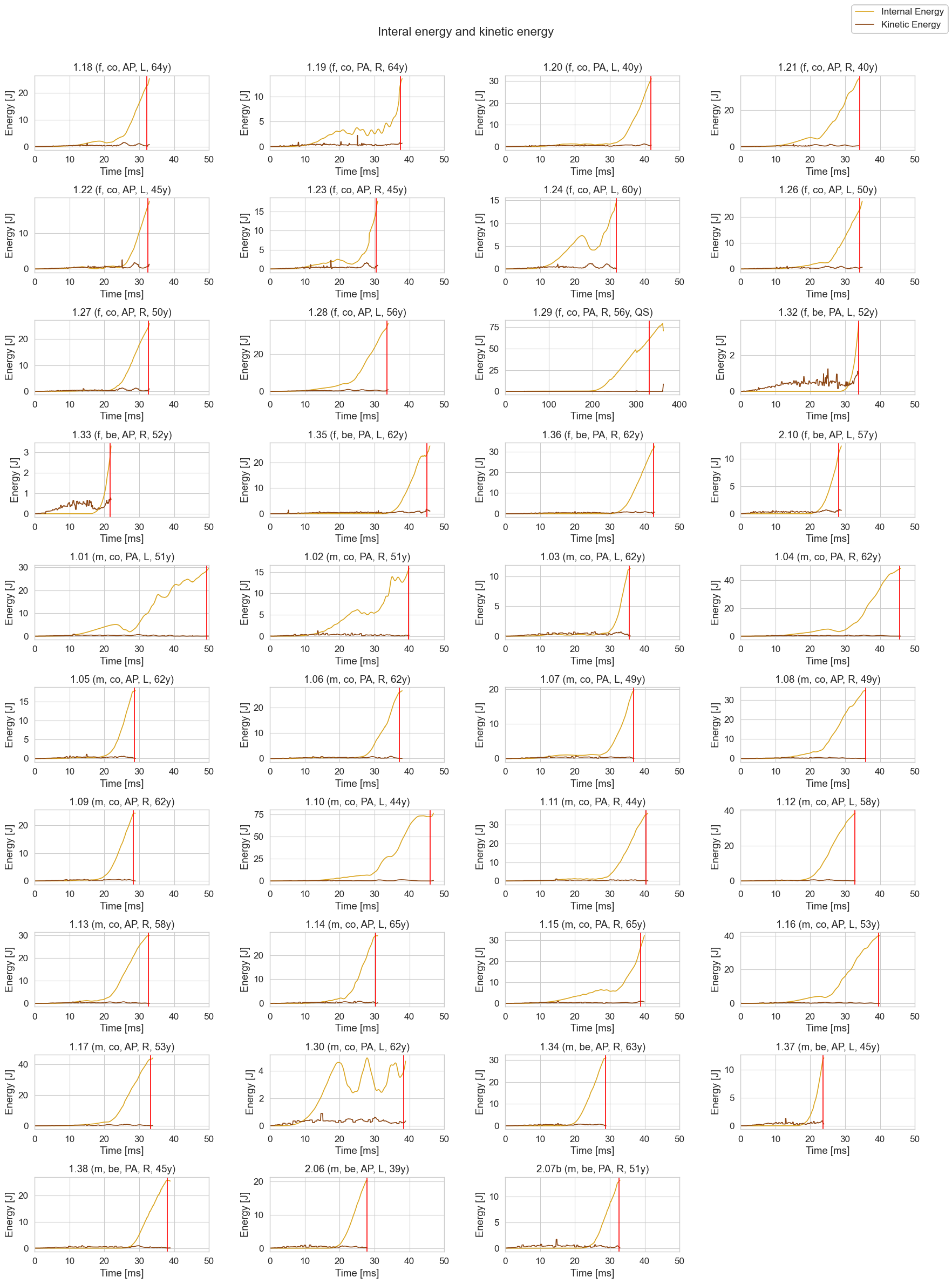
figure_title = 'Interal energy and kinetic energy'
experiment_file = None
sim_x_data = 'MODEL', 'Internal_Energy', 'time'
sim_y_data = 'MODEL', 'Internal_Energy', 'energy'
sim_x_data2 = 'MODEL', 'Kinetic_Energy', 'time'
sim_y_data2 = 'MODEL', 'Kinetic_Energy', 'energy'
sim_name1_legend = 'Internal Energy'
sim_name2_legend = 'Kinetic Energy'
x_label = 'Time [ms]'
y_label = 'Energy [J]'
x_lim = [0, 50]
y_lim = None
sign_swap_exp_data = 1
sign_swap_sim_data = 1
filename_save = 'results/figures/Ivarsson__interal_energy__kinetic_energy__time.svg'
create_subplots(experiment_file, figure_title, sim_x_data, sim_y_data, sim_x_data2, sim_y_data2, sim_name1_legend,
sim_name2_legend, x_label, y_label, x_lim, y_lim, sign_swap_exp_data, sign_swap_sim_data, filename_save)
<>:103: SyntaxWarning: "is not" with a literal. Did you mean "!="?
<>:103: SyntaxWarning: "is not" with a literal. Did you mean "!="?
C:\Users\klugcor\AppData\Local\Temp\ipykernel_9508\106710733.py:103: SyntaxWarning: "is not" with a literal. Did you mean "!="?
  if i is not '1_29':
Find values at time of evaluation#
Show code cell content
def find_value_at_time_of_evaluation(value_x, value_y):
    list = []
    counter = 0
    for i in simulation_list:
        processed_data_path = os.path.join(processed_data_dir, i).replace('\\', '/')
        simData = pd.read_csv(os.path.join(processed_data_path, dynasaur_output_file_name),
                              delimiter=';', na_values='-', header = [0,1,2,3])
        x = simData[value_x]
        y = simData[value_y]
        x = np.array(x).flatten()
        y = np.array(y).flatten()
        res = np.interp(time_for_strain_eval[counter], x, y)
        res = np.round(res, decimals=5)
        list.append(res)
        counter += 1
    return list


value_x = 'BONES', 'Femur_Cortical_L_MPS_history', 'time'
value_y = 'BONES', 'Femur_Cortical_L_MPS_history', 'strain'
MPS_list = find_value_at_time_of_evaluation(value_x, value_y)

value_x = 'BONES', 'Femur_Cortical_L_PS99_history', 'time'
value_y = 'BONES', 'Femur_Cortical_L_PS99_history', 'strain'
PS99_list = find_value_at_time_of_evaluation(value_x, value_y)

value_x = 'FEMUR', 'Impactor_rcforc_z', 'time'
value_y = 'FEMUR', 'Impactor_rcforc_z', 'force'
force_list = find_value_at_time_of_evaluation(value_x, value_y)

value_x = 'FEMUR', 'Impactor_nodout_z', 'time'
value_y = 'FEMUR', 'Impactor_nodout_z', 'displacement'
displ_list = find_value_at_time_of_evaluation(value_x, value_y)
displ_list = [i * (-1) for i in displ_list]


sheet1 = ipysheet.sheet(rows=len(simulation_list), columns=6, column_headers=False, row_headers=False)

column0 = column(0, simulation_list)
column1 = column(1, time_for_strain_eval, numeric_format = '0.0', read_only=True)
column2 = column(2, force_list, numeric_format = '0.00', read_only=True)
column2 = column(3, displ_list, numeric_format = '0.00', read_only=True)
column4 = column(4, MPS_list, numeric_format = '0.00000', read_only=True)
column5 = column(5, PS99_list, numeric_format = '0.00000', read_only=True)

sheet1.column_headers=['Simulation', 'Time of evaluation [ms]', 'Force at evaluation [kN]',
                       'Displacement at evaluation [mm]', 'MPS [-]', 'PS99 [-]']
display(sheet1)


sheet2=ipysheet.sheet(rows=len(simulation_list), colums=2, column_headers=False, row_headers=False)
column0 = column(0, simulation_list)
column1 = column(1, MPS_list, numeric_format='0.00000')
column2 = column(2, PS99_list, numeric_format='0.00000')
sheet2.column_headers=['Simulation', 'MPS', 'PS99']
df = ipysheet.to_dataframe(sheet2)

# include male and female, exclude outliner
exclude_simulation_list = ["1_10", "1_29", "1_30","1_32", "1_33"]

# for female IRC: exclude male from exported strain sheet
#exclude_simulation_list = ["1_01", "1_02", "1_03", "1_04", "1_05", "1_06", "1_07", "1_08", "1_09", "1_10", "1_11", "1_12", "1_13", "1_14", "1_15", "1_16", "1_17", "1_30", "1_34", "1_37", "1_38", "2_06", "2_07b"]

#for male IRC: exclude female from exported strain sheet
#exclude_simulation_list = ["1_18", "1_19", "1_20", "1_21", "1_22", "1_23", "1_24", "1_26", "1_27", "1_28", "1_29", "1_32", "1_33", "1_35", "1_36", "2_10"]

for i in range(len(exclude_simulation_list)):
    df.drop(df.loc[df['Simulation'] == exclude_simulation_list[i]].index, inplace=True)
df.to_csv('data/processed/strain_sheet_for_IRC.csv', index=None, sep=';', mode='w')
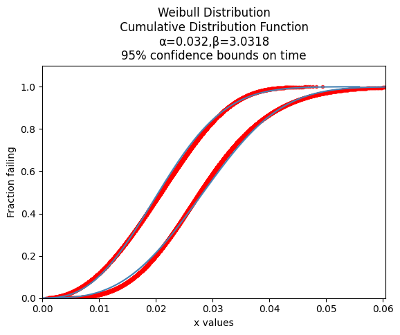
Injury Risk Curves#
Show code cell source
import os
import sys
import scipy
import numpy as np
import pandas as pd
import matplotlib.pyplot as plt
import scipy.stats as stats
from lifelines import WeibullFitter
from autograd import jacobian as jac
import autograd.numpy as anp
from reliability.Distributions import Weibull_Distribution
from reliability.Fitters import Fit_Weibull_2P, Fit_Weibull_3P
from reliability.Probability_plotting import plot_points
import matplotlib.pyplot as plt
df_strains = pd.read_csv('data/processed/strain_sheet_for_IRC.csv', sep = ";")
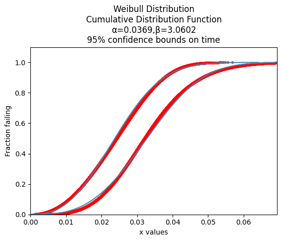
def confidence_interval_weibul_time(CI, alpha, beta, Cov_alpha_beta, alpha_SE, beta_SE):
Y= np.arange(0.0001,0.9999,0.0001)
Z = -stats.norm.ppf((1 - CI) / 2) # converts CI to Z
v_lower = v(Y, alpha, beta) - Z * (var_v(Y, alpha, beta, Cov_alpha_beta, alpha_SE, beta_SE) ** 0.5)
v_upper = v(Y, alpha, beta) + Z * (var_v(Y, alpha, beta, Cov_alpha_beta, alpha_SE, beta_SE) ** 0.5)
t_lower = np.exp(v_lower) # transform back from ln(t)
t_upper = np.exp(v_upper)
yy = 1 - Y
df = pd.DataFrame(columns=('yy', 't_lower', 't_upper'))
df.yy = yy
df.t_lower = t_lower
df.t_upper = t_upper
#print(df)
print('------Lower----------')
weibull_fit_lower = Fit_Weibull_2P(failures=list(df.t_lower), show_probability_plot=False, print_results=True,
CI=0.95, CI_type="time")
print('------Upper----------')
weibull_fit_upper = Fit_Weibull_2P(failures=list(df.t_upper), show_probability_plot=False, print_results=True,
CI=0.95, CI_type="time")
weibull_fit_lower.distribution.CDF(label='Fitted distribution', color='steelblue')
plot_points(failures=list(df.t_lower),func='CDF',label='Failure data', color='red', alpha=0.7)
weibull_fit_upper.distribution.CDF(label='Fitted distribution', color='steelblue')
plot_points(failures=list(df.t_upper),func='CDF',label='Failure data', color='red', alpha=0.7)
plt.show()
def u(t, alpha, beta): # u = ln(-ln(R))
return beta * (anp.log(t) - anp.log(alpha)) # weibull SF linearized
def v(R, alpha, beta): # v = ln(t)
return (1 / beta) * anp.log(-anp.log(R)) + anp.log(
alpha
) # weibull SF rearranged for t
def var_u(v, alpha, beta, Cov_alpha_beta, alpha_SE, beta_SE): # v is time
du_da = jac(u, 1) # derivative wrt alpha (bounds on reliability)
du_db = jac(u, 2) # derivative wrt beta (bounds on reliability)
return (
du_da(v, alpha, beta) ** 2 * alpha_SE ** 2
+ du_db(v, alpha, beta) ** 2 * beta_SE ** 2
+ 2
* du_da(v, alpha, beta)
* du_db(v, alpha, beta)
* Cov_alpha_beta
)
def var_v(u, alpha, beta, Cov_alpha_beta, alpha_SE, beta_SE): # u is reliability
dv_da = jac(v, 1) # derivative wrt alpha (bounds on time)
dv_db = jac(v, 2) # derivative wrt beta (bounds on time)
return (
dv_da(u, alpha, beta) ** 2 * alpha_SE ** 2
+ dv_db(u, alpha, beta) ** 2 * beta_SE ** 2
+ 2
* dv_da(u, alpha, beta)
* dv_db(u, alpha, beta)
* Cov_alpha_beta
)
strains = ['MPS', 'PS99']
for i in range(len(strains)):
print('--------------------------------------------------------------------------------------')
print (strains[i])
strain_list = list(df_strains[strains[i]])
print('--------------------------------------------------------------------------------------')
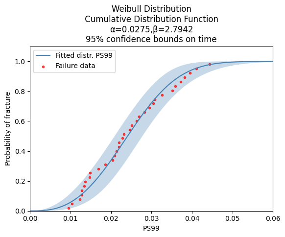
weibull_fit = Fit_Weibull_2P(failures=strain_list, show_probability_plot=False, print_results=True,
CI=0.95, CI_type="time")
label = 'Fitted distr. ' + strains[i]
weibull_fit.distribution.CDF(label=label, color='steelblue')
plot_points(failures=strain_list, func='CDF', label='Failure data', color='red',alpha=0.7)
plt.legend()
plt.xlabel(strains[i])
plt.xlim([0, 0.06])
plt.ylabel('Probability of fracture')
filepath = 'results/figures/weibull_{}_fit.svg'.format(strains[i])
plt.savefig(filepath, format='svg', bbox_inches='tight')
plt.show()
confidence_interval_weibul_time(0.95, weibull_fit.alpha, weibull_fit.beta, weibull_fit.Cov_alpha_beta,
weibull_fit.alpha_SE, weibull_fit.beta_SE)
--------------------------------------------------------------------------------------
MPS
--------------------------------------------------------------------------------------
Results from Fit_Weibull_2P (95% CI):
Analysis method: Maximum Likelihood Estimation (MLE)
Optimizer: TNC
Failures / Right censored: 34/0 (0% right censored)

Parameter  Point Estimate  Standard Error  Lower CI  Upper CI
    Alpha       0.0317518      0.00203919 0.0279963  0.036011
     Beta         2.82072        0.379688   2.16662   3.67229

Goodness of fit    Value
 Log-likelihood  106.119
           AICc -207.851
            BIC -205.185
             AD 0.671476

------Lower----------
Results from Fit_Weibull_2P (95% CI):
Analysis method: Maximum Likelihood Estimation (MLE)
Optimizer: L-BFGS-B
Failures / Right censored: 9998/0 (0% right censored)

Parameter  Point Estimate  Standard Error  Lower CI  Upper CI
    Alpha        0.027331     0.000110258 0.0271157 0.0275479
     Beta          2.6031       0.0208747   2.56251   2.64434

Goodness of fit    Value
 Log-likelihood  31859.5
           AICc -63714.9
            BIC -63700.5
             AD  13.3172

------Upper----------
Results from Fit_Weibull_2P (95% CI):
Analysis method: Maximum Likelihood Estimation (MLE)
Optimizer: L-BFGS-B
Failures / Right censored: 9998/0 (0% right censored)

Parameter  Point Estimate  Standard Error  Lower CI  Upper CI
    Alpha       0.0369252     0.000127483 0.0366762 0.0371759
     Beta         3.06022       0.0230068   3.01546   3.10565

Goodness of fit    Value
 Log-likelihood  30485.8
           AICc -60967.7
            BIC -60953.2
             AD  20.7649
--------------------------------------------------------------------------------------
PS99
--------------------------------------------------------------------------------------
Results from Fit_Weibull_2P (95% CI):
Analysis method: Maximum Likelihood Estimation (MLE)
Optimizer: TNC
Failures / Right censored: 34/0 (0% right censored)

Parameter  Point Estimate  Standard Error  Lower CI  Upper CI
    Alpha       0.0274591      0.00178048 0.0241821 0.0311803
     Beta         2.79418        0.376437   2.14574   3.63856

Goodness of fit    Value
 Log-likelihood  110.804
           AICc -217.222
            BIC -214.556
             AD 0.673409
------Lower----------
Results from Fit_Weibull_2P (95% CI):
Analysis method: Maximum Likelihood Estimation (MLE)
Optimizer: L-BFGS-B
Failures / Right censored: 9998/0 (0% right censored)

Parameter  Point Estimate  Standard Error  Lower CI  Upper CI
    Alpha       0.0236013     9.61276e-05 0.0234136 0.0237905
     Beta         2.57831       0.0206764    2.5381   2.61915

Goodness of fit    Value
 Log-likelihood  33252.7
           AICc -66501.5
            BIC   -66487
             AD  13.3444

------Upper----------
Results from Fit_Weibull_2P (95% CI):
Analysis method: Maximum Likelihood Estimation (MLE)
Optimizer: TNC
Failures / Right censored: 9998/0 (0% right censored)

Parameter  Point Estimate  Standard Error  Lower CI  Upper CI
    Alpha       0.0319805     0.000111448 0.0317628 0.0321996
     Beta         3.03176       0.0227917   2.98742   3.07677

Goodness of fit    Value
 Log-likelihood  31846.9
           AICc -63689.7
            BIC -63675.3
             AD  20.8199