Tibia shaft (Harden 2021)#
Validation model information#
Performed by: Elena Weissenbacher, Nico Erlinger
Reviewed by: Corina Klug
Added to VIVA+ Validation Catalog on: 2022-11-31
Last modified: 2023-11-23
Model version (this notebook run for): 0.3.2
The Jupyter notebooks are licensed under Creative Commons Attribution 4.0 International License 
Experiments by Harden et al. (2021)#
Harden, A.; Kang, Y. S.; Hunter, R.; Bendig, A.; Bolte, J.; Eckstein, N.; Smith, A.; Agnew, A. 2021. Preliminary Sex-specific Relationships between Peak Force and Cortical Bone Morphometrics in Human Tibiae Subjected to Lateral Loading. In Proccedings of the IRCOBI Conference 2021, Online. http://www.ircobi.org/wordpress/downloads/irc21/pdf-files/2133.pdf
Summary#
Five female and five male isolated tibiae were subjeted to four-point bending.
Information on the subjects/specimens#
Test number |
Sex |
Donor age [yr] |
Mechanical span [mm] |
|---|---|---|---|
Tib-001 |
M |
64 |
191 |
Tib-002 |
M |
63 |
188 |
Tib-003 |
M |
77 |
166 |
Tib-004 |
F |
84 |
161 |
Tib-005 |
F |
86 |
161 |
Tib-006 |
F |
102 |
160 |
Tib-007 |
M |
73 |
165 |
Tib-008 |
M |
74 |
183 |
Tib-009 |
F |
85 |
162 |
Tib-010 |
F |
89 |
148 |
Loading and Boundary Conditions#
A constant impactor velocity of 6 m/s was prescribed. Mechanical span of the potting was adjusted to experimental data for each simulation.
Experimental responses#
The force-time history plots published by Harden et al. (2021) were digitised with WebPlotDigitizer v4.4 (https://automeris.io/WebPlotDigitizer).
Results#
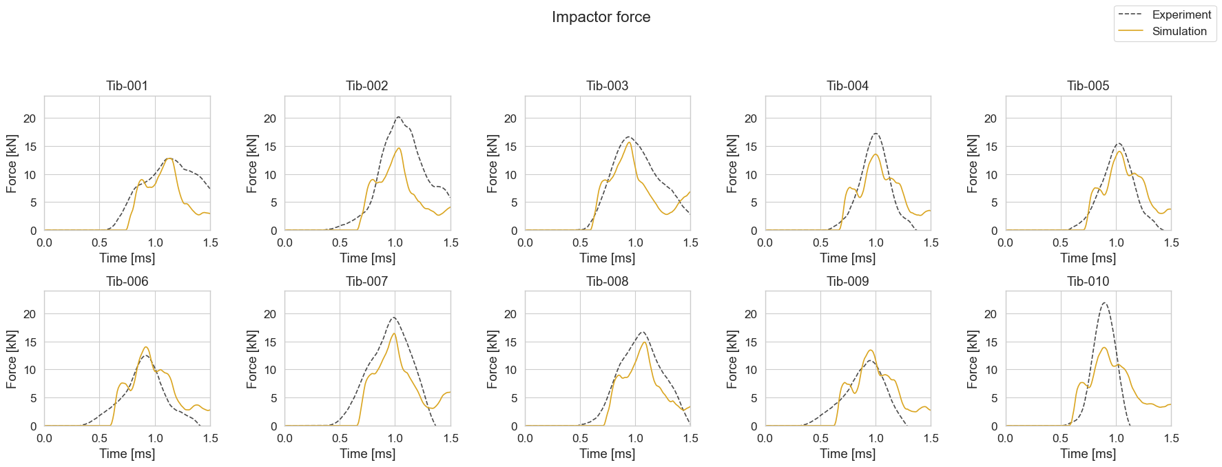
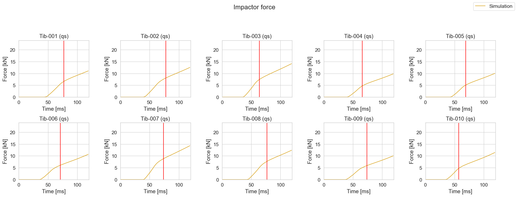
Impactor force plots#
Show code cell source
create_subplots(
figure_title = 'Impactor force',
sim_x_data = ('TIBIA', 'Contact_Force_proximal_z', 'time'),
sim_y_data = ('TIBIA', 'Contact_Force_proximal_z', 'force'),
sim_data_for_calculation_y = ('TIBIA', 'Contact_Force_distal_z', 'force'),
sim_name1_legend = 'Simulation',
exp_x_data = ('time', 'ms'),
exp_y_data = ('force', 'kN'),
exp_name1_legend = 'Experiment',
x_label = ('Time [ms]'),
y_label = ('Force [kN]'),
x_lim = [0, 1.5],
y_lim = [0, 24],
filename_save = figure_dir + '/Harden_2021_force_time.svg' )
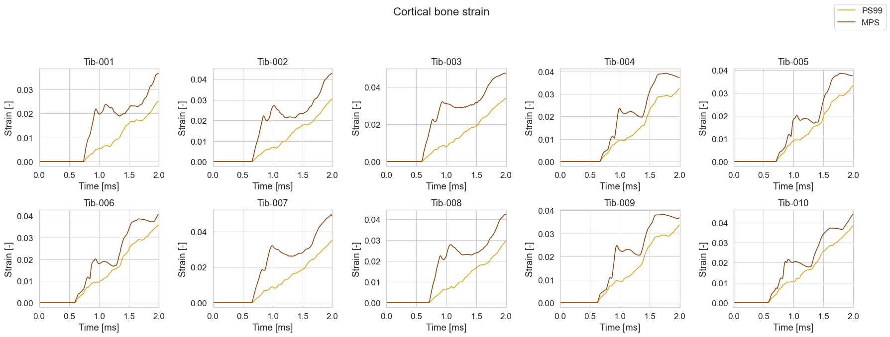
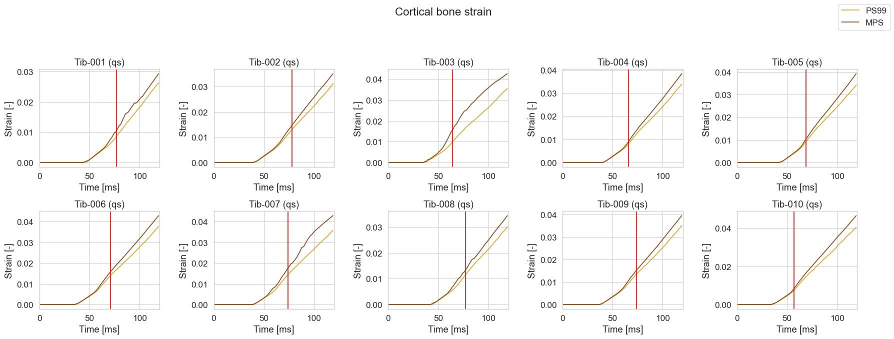
Plot strain-time histories#
Show code cell source
create_subplots(
figure_title = 'Cortical bone strain',
sim_x_data = ('BONES', 'Tibia_Cortical_R_PS99', 'time'),
sim_y_data = ('BONES', 'Tibia_Cortical_R_PS99', 'strain'),
sim_x_data2 = ('BONES', 'Tibia_Cortical_R_MPS', 'time'),
sim_y_data2 = ('BONES', 'Tibia_Cortical_R_MPS', 'strain'),
sim_name1_legend = 'PS99',
sim_name2_legend = 'MPS',
x_label = 'Time [ms]',
y_label = 'Strain [-]',
x_lim = [0, 2],
filename_save = figure_dir + '/Harden_2021_tibia_strain_time.svg')
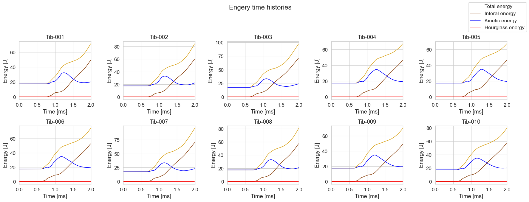
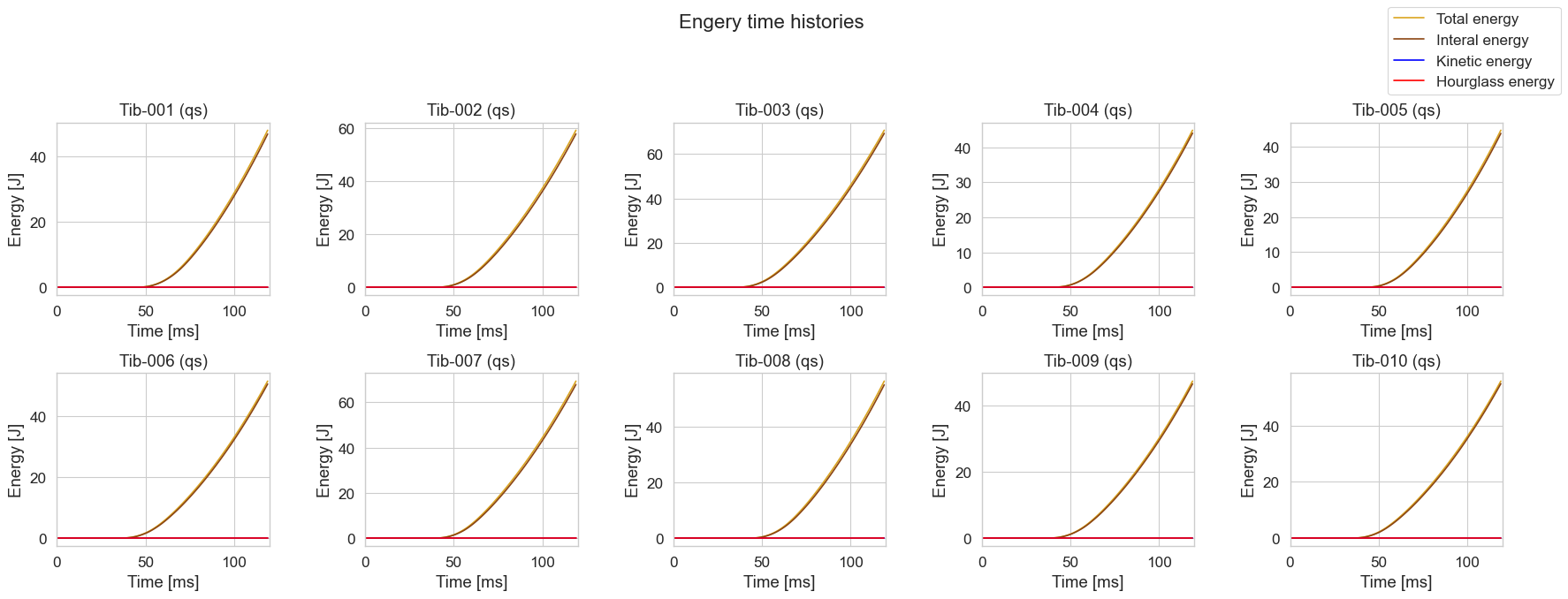
Engergy-time plots#
Show code cell source
create_subplots(
figure_title = 'Engery time histories',
sim_x_data = ('MODEL', 'Total_Energy', 'time'),
sim_y_data = ('MODEL', 'Total_Energy', 'energy'),
sim_x_data2 = ('MODEL', 'Internal_Energy', 'time'),
sim_y_data2 = ('MODEL', 'Internal_Energy', 'energy'),
sim_x_data3 = ('MODEL', 'Kinetic_Energy', 'time'),
sim_y_data3 = ('MODEL', 'Kinetic_Energy', 'energy'),
sim_x_data4 = ('MODEL', 'Hourglass_Energy', 'time'),
sim_y_data4 = ('MODEL', 'Hourglass_Energy', 'energy'),
sim_name1_legend = 'Total energy',
sim_name2_legend = 'Interal energy',
sim_name3_legend = 'Kinetic energy',
sim_name4_legend = 'Hourglass energy',
x_label = 'Time [ms]',
y_label = 'Energy [J]',
x_lim = [0, 2],
filename_save = figure_dir + '/Harden_2021_time_histories.svg')
ISO18571 objective rating for force-time histories#
Show code cell source
simulation_list = ['Tib-001','Tib-002','Tib-003','Tib-004','Tib-005','Tib-006','Tib-007','Tib-008','Tib-009','Tib-010']

def calculate_iso_score(processed_data_dir, experiment_data_file, sim_x_data, sim_y_data, sim_data_for_calculation_y, exp_x_data, exp_y_data):
    ratings = []
    for i in simulation_list:
        experimental_data = pd.read_csv(experiment_data_file, delimiter=';', header=[0,1,2,3], decimal='.')
        processed_data_path = os.path.join(processed_data_dir, i).replace('\\', '/')
        simData = pd.read_csv(os.path.join(processed_data_path, dynasaur_output_file_name),
                                    delimiter=';', na_values='-', header = [0,1,2,3])

        time_ref = np.array(experimental_data[(i,) + exp_x_data]).flatten()
        x_ref = np.array(experimental_data[(i,) + exp_y_data]).flatten()

        time_comp=np.array(simData[sim_x_data]).flatten()
        x_comp = simData[sim_y_data]

        if sim_data_for_calculation_y is not None:
            x_comp = x_comp + simData[sim_data_for_calculation_y]
        x_comp=np.array(x_comp).flatten()

        time_comp = np.delete(time_comp,np.s_[150:])
        x_comp = np.delete(x_comp, np.s_[150:])

        ind_nan = []
        ind_nan = np.where(np.isnan(x_ref))

        if len(ind_nan[0]) > 0:
            x_ref = x_ref[0:ind_nan[0][0]-1]
            x_time_ref = time_ref[0:ind_nan[0][0]-1]
            x_comp = x_comp[0:ind_nan[0][0]-1]
            x_time_comp = time_comp[0:ind_nan[0][0]-1]
        else:
            x_time_ref = time_ref
            x_time_comp = time_comp

        if len(x_ref) > len(x_comp):
            ind_end = len(x_comp)
            x_ref = x_ref[0:ind_end]
            x_time_ref = x_time_ref[0:ind_end]

        elif len(x_comp) > len(x_ref):
            ind_end = len(x_ref)
            x_comp = x_comp[0:ind_end]
            x_time_comp = x_time_comp[0:ind_end]

        ref = np.vstack((x_time_ref, x_ref)).T
        comp = np.vstack((x_time_comp, x_comp)).T

        iso_rating = ISO18571(reference_curve=ref, comparison_curve=comp)

        ratings.append([i,
        iso_rating.corridor_rating(),
        iso_rating.phase_rating(),
        iso_rating.magnitude_rating(),
        iso_rating.slope_rating(),
        iso_rating.overall_rating()])

    rating_array = []
    rating_array = np.append(rating_array, ratings)
    rating_array = rating_array.transpose()
    rating_array = np.reshape(rating_array, (10,6))

    return(rating_array)

iso_ratings = calculate_iso_score(
sim_x_data = ('TIBIA', 'Contact_Force_proximal_z', 'time'),
sim_y_data = ('TIBIA', 'Contact_Force_proximal_z', 'force'),
sim_data_for_calculation_y = ('TIBIA', 'Contact_Force_distal_z', 'force'),
experiment_data_file = 'data/experiment/Harden_2021_testdata.csv',
exp_x_data = ('time', 'ms'),
exp_y_data = ('force', 'kN'),
processed_data_dir = processed_data_dir
)

df = pd.DataFrame(iso_ratings, columns=['Simulation', 'Corridor', 'Phase', 'Magnitude', 'Slope', 'Overall'])
display(df)
| Simulation | Corridor | Phase | Magnitude | Slope | Overall | |
|---|---|---|---|---|---|---|
| 0 | Tib-001 | 0.678 | 0.9 | 0.742 | 0.34 | 0.668 |
| 1 | Tib-002 | 0.637 | 0.767 | 0.635 | 0.676 | 0.67 |
| 2 | Tib-003 | 0.714 | 0.833 | 0.898 | 0.599 | 0.752 |
| 3 | Tib-004 | 0.722 | 0.9 | 0.718 | 0.598 | 0.732 |
| 4 | Tib-005 | 0.757 | 0.833 | 0.824 | 0.607 | 0.756 |
| 5 | Tib-006 | 0.69 | 0.8 | 0.813 | 0.532 | 0.705 |
| 6 | Tib-007 | 0.646 | 0.9 | 0.741 | 0.655 | 0.718 |
| 7 | Tib-008 | 0.753 | 0.967 | 0.91 | 0.705 | 0.818 |
| 8 | Tib-009 | 0.601 | 0.733 | 0.712 | 0.491 | 0.628 |
| 9 | Tib-010 | 0.63 | 0.833 | 0.432 | 0.573 | 0.619 |
Quasistatic simulations#
Show code cell source
simulation_list = ['Tib-001_quasistatic','Tib-002_quasistatic','Tib-003_quasistatic','Tib-004_quasistatic','Tib-005_quasistatic',
                    'Tib-006_quasistatic','Tib-007_quasistatic','Tib-008_quasistatic','Tib-009_quasistatic','Tib-010_quasistatic']

simulation_titles = ['Tib-001 (qs)','Tib-002 (qs)','Tib-003 (qs)','Tib-004 (qs)','Tib-005 (qs)',
                    'Tib-006 (qs)','Tib-007 (qs)','Tib-008 (qs)','Tib-009 (qs)','Tib-010 (qs)']

create_subplots(
figure_title = 'Impactor force',
sim_x_data = ('TIBIA', 'Contact_Force_proximal_z', 'time'),
sim_y_data = ('TIBIA', 'Contact_Force_proximal_z', 'force'),
sim_data_for_calculation_y = ('TIBIA', 'Contact_Force_distal_z', 'force'),
sim_name1_legend = 'Simulation',
x_label = ('Time [ms]'),
y_label = ('Force [kN]'),
time_for_strain_eval =[77, 78, 64, 66, 69, 71, 74, 77, 74, 57],
x_lim = [0, 120],
y_lim = [0, 24],
filename_save = figure_dir + '/VIVA+_Harden_2021_force_time.svg' )


create_subplots(
figure_title = 'Cortical bone strain',
sim_x_data = ('BONES', 'Tibia_Cortical_R_PS99', 'time'),
sim_y_data = ('BONES', 'Tibia_Cortical_R_PS99', 'strain'),
sim_x_data2 = ('BONES', 'Tibia_Cortical_R_MPS', 'time'),
sim_y_data2 = ('BONES', 'Tibia_Cortical_R_MPS', 'strain'),
sim_name1_legend = 'PS99',
sim_name2_legend = 'MPS',
x_label = 'Time [ms]',
y_label = 'Strain [-]',
time_for_strain_eval =[77, 78, 64, 66, 69, 71, 74, 77, 74, 57],
x_lim = [0, 120],
filename_save = figure_dir + '/Harden_2021_tibia_strain_time.svg')


create_subplots(
figure_title = 'Engery time histories',
sim_x_data = ('MODEL', 'Total_Energy', 'time'),
sim_y_data = ('MODEL', 'Total_Energy', 'energy'),
sim_x_data2 = ('MODEL', 'Internal_Energy', 'time'),
sim_y_data2 = ('MODEL', 'Internal_Energy', 'energy'),
sim_x_data3 = ('MODEL', 'Kinetic_Energy', 'time'),
sim_y_data3 = ('MODEL', 'Kinetic_Energy', 'energy'),
sim_x_data4 = ('MODEL', 'Hourglass_Energy', 'time'),
sim_y_data4 = ('MODEL', 'Hourglass_Energy', 'energy'),
sim_name1_legend = 'Total energy',
sim_name2_legend = 'Interal energy',
sim_name3_legend = 'Kinetic energy',
sim_name4_legend = 'Hourglass energy',
x_label = 'Time [ms]',
y_label = 'Energy [J]',
x_lim = [0, 120],
filename_save = figure_dir + '/Harden_2021_time_histories.svg')
Strains at time of experimental peak force#
Show code cell source
def find_value_at_time_of_evaluation(value_x, value_y, time_for_strain_eval):
    list = []
    counter = 0
    for i in simulation_list:
        processed_data_path = os.path.join(processed_data_dir, i).replace('\\', '/')
        simData = pd.read_csv(os.path.join(processed_data_path, dynasaur_output_file_name),
                              delimiter=';', na_values='-', header = [0,1,2,3])
        x = simData[value_x]
        y = simData[value_y]
        x = np.array(x).flatten()
        y = np.array(y).flatten()
        res = np.interp(time_for_strain_eval[counter], x, y)
        res = np.round(res, decimals=5)
        list.append(res)
        counter += 1
    return list

simulation_list = ['Tib-001_quasistatic','Tib-002_quasistatic','Tib-003_quasistatic','Tib-004_quasistatic','Tib-005_quasistatic',
                    'Tib-006_quasistatic','Tib-007_quasistatic','Tib-008_quasistatic','Tib-009_quasistatic','Tib-010_quasistatic']

time_for_strain_eval =[77, 78, 64, 66, 69, 71, 74, 77, 74, 57]


MPS_list = find_value_at_time_of_evaluation(
value_x = ('BONES', 'Tibia_Cortical_R_MPS', 'time'),
value_y = ('BONES', 'Tibia_Cortical_R_MPS', 'strain'),
time_for_strain_eval = time_for_strain_eval
)

PS99_list = find_value_at_time_of_evaluation(
value_x = ('BONES', 'Tibia_Cortical_R_PS99', 'time'),
value_y = ('BONES', 'Tibia_Cortical_R_PS99', 'strain'),
time_for_strain_eval = time_for_strain_eval
)

df = pd.DataFrame({'MPS': MPS_list, 'PS99': PS99_list})
df.to_csv('data/processed/strain_sheet_for_IRC.csv', index=None, sep=';', mode='w')

display(df)
| MPS | PS99 | |
|---|---|---|
| 0 | 0.01051 | 0.00864 |
| 1 | 0.01461 | 0.01300 |
| 2 | 0.01536 | 0.00981 |
| 3 | 0.00915 | 0.00819 |
| 4 | 0.01040 | 0.00925 |
| 5 | 0.01578 | 0.01404 |
| 6 | 0.01753 | 0.01436 |
| 7 | 0.01319 | 0.01141 |
| 8 | 0.01531 | 0.01362 |
| 9 | 0.00835 | 0.00752 |
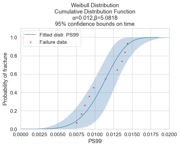
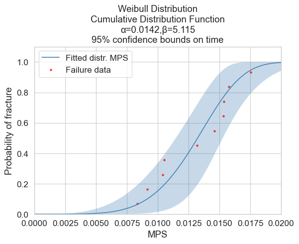
Fracture risk curve#
Show code cell source
import os
import numpy as np
import pandas as pd
import matplotlib.pyplot as plt
from reliability.Fitters import Fit_Weibull_2P
from reliability.Probability_plotting import plot_points


df_strains = pd.read_csv('data/processed/strain_sheet_for_IRC.csv', sep = ";")

strains = ['MPS', 'PS99']

for i in range(len(strains)):
    print('--------------------------------------------------------------------------------------')
    print (strains[i])
    strain_list = list(df_strains[strains[i]])
    print('--------------------------------------------------------------------------------------')
    weibull_fit = Fit_Weibull_2P(failures=strain_list, show_probability_plot=False, print_results=False,CI=0.95, CI_type="time")
    label = 'Fitted distr. ' + strains[i]
    weibull_fit.distribution.CDF(label=label, color='steelblue')
    plot_points(failures=strain_list, func='CDF', label='Failure data', color='red',alpha=0.7)
    plt.legend()
    plt.xlabel(strains[i])
    plt.xlim([0, 0.02])
    plt.ylabel('Probability of fracture')
    filepath = figure_dir + '/weibull_{}_fit.svg'.format(strains[i])
    plt.savefig(filepath, format='svg', bbox_inches='tight')
    plt.show()
--------------------------------------------------------------------------------------
MPS
--------------------------------------------------------------------------------------
--------------------------------------------------------------------------------------
PS99
--------------------------------------------------------------------------------------